Contents

Introduction

These are my notes for the seminars that happen in the Theory Group at The University of Toronto. Many thanks to Professor Allan Borodin for allowing me to attend the Theory Group seminars and helping out.

A PDF of these notes is available at https://rishit-dagli.github.io/cs-theory-notes/main.pdf. An online version of these notes are available at https://rishit-dagli.github.io/cs-theory-notes.

The Theory Group focuses on theory of computation. The group is interested in using mathematical techniques to understand the nature of computation and to design and analyze algorithms for important and fundamental problems.

The members of the theory group are all interested, in one way or another, in the limitations of computation: What problems are not feasible to solve on a computer? How can the infeasibility of a problem be used to rigorously construct secure cryptographic protocols? What problems cannot be solved faster using more machines? What are the limits to how fast a particular problem can be solved or how much space is needed to solve it? How do randomness, parallelism, the operations that are allowed, and the need for fault tolerance or security affect this?

1 Lower Bounds for Locally Decodable Codes from Semirandom CSP Refutation

7th October 2022

The related paper: Combinatorial lower bounds for 3-query LDCs by Alrabiah et al. [1]. Seminar by Peter Manohar. [2] [3]

1.1 Abstract

A code $C$ is a q-locally decodable code (q-LDC) if one can recover any chosen bit $b_i$ of the $k$-bit message b with good confidence by randomly querying the $n$-bit encoding x on at most $q$ coordinates. Existing constructions of $2$-LDCs achieve blocklength $n=\mathit{exp}(O(k))$, and lower bounds show that this is in fact tight. However, when $q=3$, far less is known: the best constructions have $n=\mathit{subexp}(k)$, while the best known lower bounds, that have stood for nearly two decades, only show a quadratic lower bound of $n\ge \mathrm{\Omega }(k^2)$ on the blocklength.

In this talk, we will survey a new approach to prove lower bounds for LDCs using recent advances in refuting semirandom instances of constraint satisfaction problems. These new tools yield, in the $3$-query case, a near-cubic lower bound of $n\ge \tilde{\mathrm{\Omega }}(k^3)$, improving on prior work by a polynomial factor in $k$.

1.2 Locally Decodable Codes

Take codes $b\in {0,1}^k\to x\in {0,1}^n$

Codes $x$ are read by the decoder, $i\in [k]$, $\widehat{b_i}\in 0,1$

Ask the question, what is the best possible rate for a $q$-LDC given a $q$?

Focus on the case $q=3$, we have gotten better bounds:

In [1], they show that a better minimum bound can be found than these existing ones for $q=3$:

The main result is that:

Semi-random CSP refutation comes to our aid to prove this! The intuitive way to put this theorem is that $q$-LDC lower bound is same as refuting ”LDC” $q$-XOR.

1.3 How to prove the Theorem

The idea:

• $q$-LDC lower bound is same as refuting ”LDC” $q$-XOR

  • CSP Refutation
• Proof of existing $q$-LDC lower bound for $q$ even
• Proof sketch of $k^3$ lower bound

1.4 Normally Decodable Codes

We can see that the decoder we have can arbitrary but WLOG we can assume there are $q$-unif hypergraphs $H_1,H_2,\cdots H_k$ where every $H_i$ is such that:

We can also see that:

Each $H_i$ is a matching such that $\left|H_i\right|\ge \mathit{\delta n}$

and, $\mathit{Dec}(i)$ picks $C\leftarrow H_i$ and outputs ${\sum <!--\; FUNCTION\; APPLICATION\; -->}_{j\in C}{x}_j$

One such example is the Hadmard code:

Can think of this as $v$ and $v+e_i$ are connected.

Matching vector codes are $\approx {\mathbb{Z}}_m^h$

1.5 Proof: Going from LDC to XOR

We suppose that our code is linear and that there exists $q$-unif hypergraphs $H_1,H_2,\cdots H_k$.

We also know that:

Each $H_i$ is a matching such that $\left|H_i\right|\ge \mathit{\delta n}$

and, $\mathit{Dec}(i)$ picks $C\leftarrow H_i$ and outputs ${\sum <!--\; FUNCTION\; APPLICATION\; -->}_{j\in C}{x}_j$

So, we start by considering a $q$-XOR instance ${\psi }_b$:

We can write down the maximum fraction of satisfiable constraints: $\mathit{val}({\psi }_b)=1$ for any $b\in {0,1}^k$.

It is sufficient now if we can argue that ${\psi }_b$ is unsat with high probability for some random $b$ when $n\ll k^{\frac{q}{q-2}}$.

Now we need to refute XOR, there are many ways to argue unsatisfiability of an XOR instance. One reason why we can not use probablistic approaches here is that ${\psi }_b$ only has $k$ bits of randomness.

One way we can have some success here is to use a refutation algorithm

With this the guarantee then would be $\mathit{val}(\psi )\le \mathit{algval}(\psi )$ which is similar to saying that if $\mathit{algval}(\psi )<1$ then $A$ refutes $\psi$. The ideal goal would be to refute random $\psi$ with $m$ constraints with high probability

However, we take a look at semi-random XOR. Our refutation algorithm and the guarantee will still be the same:

with the guarantee that $\mathit{val}(\psi )\le \mathit{algval}(\psi )$.

So, now we generate semi-random $\mathit{\psi w}∕m$ constraints:

• The worst case would be random $q$-unif hypergraph
• Random RHS $b_c$ for each $C\in H$

The equation we have is:

And we also already know that

And, $\mathit{xj}=b_i,i\in [k],C\in H_i$.

${\psi }_b$ is almost semi-random.

Thus, we have shown 1 Part 1 of Proof.

1.6 Proof: Existing $q$-LDC lower bound for $q$ even

$q$-LDC XOR instance ${\psi }_b$ is encoded by:

• $q$-uniform hypergraph matchings $\{H_1\cdots H_k\}$
• right-hand sides are random $b_i\in \{\pm 1\}$
• We have constraints ${\prod <!--\; FUNCTION\; APPLICATION\; -->}_{j\in C}{x}_j=b_i$ for all $i$ and $C\in H_i$

We now have a goal to argue that ${\psi }_b$ unsat with high probability for random when $b$ when $n\ll k^{q∕(q-2)}$

frac. constraints satisfied by $x\in {\{\pm 1\}}^n$ is $\frac{1}{2}+\frac{f(x)}{2}$.

Here $f(x)$ is:

This makes our goal to be to certify with high probability that:

We will now try to refute ${\psi }_b$. With Equation 5 and Equation 6 to refute ${\psi }_b$ is like showing:

$\mathit{\text{ when }}n\ll k^{\frac{q}{q-2}}$.

The idea is to design a matrix $A\in {ℝ}^{N\times N}$ so that:

As shown by Wein et al. [4] the matrix $A$ can be indexed by

Assign $x\mapsto y$ such that $y^T\mathit{Ay}\propto f(x)$

and $y_s:={\prod <!--\; FUNCTION\; APPLICATION\; -->}_{j\in S}{x}_j$ which is simply the tensor product.
 

We need to now be able to answer how to set $A(S,T)$

Which shows that we are actually using symmetric difference here.

We say that if $S\oplus T=C\in h_i$ then ${\prod <!--\; FUNCTION\; APPLICATION\; -->}_{j\in S\oplus T}{x}_j=b_i$

$\Rightarrow A(S,T)=b_i$ if $S\oplus T=C\in H_i$

Here $D=$ number of $S,T$ where $S\oplus T=C$.

Simplifying an earlier statement we can also say from here that: $A_C(S,T)=1$ if $S\oplus T=C$.

For which $A_i={\sum <!--\; FUNCTION\; APPLICATION\; -->}_{C\in h_i}{A}_C$ and $A={\sum <!--\; FUNCTION\; APPLICATION\; -->}_{i=1}^k{b}_i{A}_i$

Set $y_S:={\prod <!--\; FUNCTION\; APPLICATION\; -->}_{j\in S}{x}_j$

$y^T\mathit{Ay}=\mathit{Dmf}(x)\Rightarrow \mathit{Dmf}(x)\le \left|\right|A|{\text{|}}_{\infty \to 1}$

Note that the way we defined $D$ here it only depends on $\left|C\right|=q$, we can say:

Also we know $A_c\in {ℝ}^{N\times N}$ and $N=\left(\genfrac{}{}{0ex}{}{n}{l}\right)$.

We have already proven that $\left|\right|A|{\text{|}}_{\infty \to 1}\ge \mathit{Dm}\underset{x}{\max <!--\; FUNCTION\; APPLICATION\; -->}f(x)\ge \mathit{Dm}\ge \mathit{D\delta nk}$

It is also interesting to note that $\left|\right|A|{\text{|}}_{\infty \to 1}\le N|\left|A\right|{\text{|}}_2$ and we still need to be able to show that with high probability that $\left|\right|A|{\text{|}}_{\infty \to 1}$ is not too large.

Matrix Bernstein: with high probability over $b_i$, $\left|\right|A|{\text{|}}_2\le △\sqrt{\mathit{kl}}$ where $\text{△}$ is the maximum number of 1’s in a row in any $A_i$.

Expected number of 1’s per row is $\mathit{\delta n}\frac{D}{N}\sim n{(\frac{l}{n})}^{q∕2}$.

We can optimistically suppose that $△\sim n{(\frac{l}{n})}^{q∕2}$ however this also needs $l\ge n^{1-2∕q}$.

Then $D\cdot \mathit{\delta nk}\le \left|\right|A|{\text{|}}_{\infty \to 1}\le N△\sqrt{\mathit{kl}}$

$\Rightarrow k\le l$ since $△\sim \mathit{\delta n}\frac{D}{N}$

Now take $l=n^{1-2∕q}\Rightarrow k^{q∕(q-2)}\le n$

So, $△=\frac{2l}{q}$

Because $H_i$ are matchings, a random row will have only $\approx \frac{\mathit{\delta nD}}{N}$ 1’s.

The idea now is to prune off all the bad rows or columns in A to get B such that:

And, ${\text{△}}_B\sim \mathit{\delta n}{(\frac{l}{n})}^{q∕2}$

And now we can just use $B$ instead which will prove $q$-LDC lower bound for $q$ even.

1.7 Proof: $k^3$ lower bound

Recall, $q$-LDC XOR instance ${\psi }_b$ is encoded by:

• $q$-uniform hypergraph matchings $\{H_1\cdots H_k\}$
• right-hand sides are random $b_i\in \{\pm 1\}$
• We have constraints ${\prod <!--\; FUNCTION\; APPLICATION\; -->}_{j\in C}{x}_j=b_i$ for all $i$ and $C\in H_i$

The goal is argue that ${\psi }_b$ is unsatisfiable with high probability for random $b$. And the idea is to design a matrix $A\in {ℝ}^{N\times N}$ so that:

The previous approach fails because the $A$ from before requires $q$ to be even.

One attempt is to represent rows as $\left|S\right|=l$ and columns as $\left|T\right|=l+1$. However this will only get us to $k\le \sqrt{n}$.

We need to derive more constraints, using $C_i\oplus C_j$ get us to $\mathit{nk}$ constraints so each $n_j$ is in $\approx k$ constraints $\Rightarrow$ new $n{k}^2$ constraints.

The matrix $A$ is indexed by $S$, $A(S,T)=b_i{b}_j$. The calculation is now:

An optimist approach is $△\sim \mathit{Nk}\frac{D}{N}=\mathit{nk}{(\frac{l}{n})}^2$

$\Rightarrow l\ge \sqrt{\frac{n}{k}}$

$\Rightarrow k\le n\Rightarrow k^3\le n$

The row pruning tricks would still work provided that any $\{u,v\}$ is in at most $\mathit{polylog}(n)$ constraints.

1.8 Conclusion

This proof for $q=3$ is not generalizable for all odd $q$ and neither is a reduction to $2$-LDC. This is particularly true because of the row pruning step.

2 Algorithms for the ferromagnetic Potts model on expanders

14th October 2022

The related paper: Algorithms for the ferromagnetic Potts model on expanders by Carlson et al. [5]. Seminar by Aditya Potukuchi.

2.1 Abstract

The ferromagnetic Potts model is a canonical example of a Markov random field from statistical physics that is of great probabilistic and algorithmic interest. This is a distribution over all $1$-colorings of the vertices of a graph where monochromatic edges are favored. The algorithmic problem of efficiently sampling approximately from this model is known to be #BIS-hard, and has seen a lot of recent interest. I will outline some recently developed algorithms for approximately sampling from the ferromagnetic Potts model on d-regular weakly expanding graphs. This is achieved by a significantly sharper analysis of standard ”polymer methods” using extremal graph theory and applications of Karger’s algorithm to count cuts that may be of independent interest. I will give an introduction to all the topics that are relevant to the results.

2.2 The Ferromagnetic Potts Model

We start by defining some basic notation:

• $G$: finite graph on vertices $V$
• $q\in \mathbb{N}$, we are interested in $q$-colourings of the vertices in $G$
• $m(\chi )$: number of monochromatic edges induced by a colouring $\chi$
• Distribution on colourings given by $p(\chi )\propto \mathit{exp}(\beta \cdot m(\chi ))$
• $\beta \in ℝ$: parameter, inverse temperature

Notice that for $\beta <0$ it means that we take the antiferromagnetic case. Here we talk more about when $\beta >0$ meaning it is ferromagnetic.

This could have quite some applications:

• Modelling: Social networks, physics, chemistry, etc
• Markov Random field: Probabilistic Inference
• Connection to UGC Coulson et al. [6]
• and more.

2.3 The Problem

we know $p(\chi )\propto \mathit{exp}(\beta \cdot m(\chi ))$

Now for $\beta =0$ it means that we are doing a uniform $q$-coloring of $V$

For $\beta =-\infty$ we do a uniform proper coloring of $G$

What we need to do is given $G$ and $\beta$, efficiently sample a coloring from this distribution.

We add the normalizing factor here:

Now we can also say,

A partition function of the model/distribution is very important for this POV.

Our problem is that given $G$ and $\beta$ we want to efficiently sample a color distribution. We give 2 facts:

1. It is enough to compute $Z_G(q,\beta )$
2. #P-hard

We now modify the problem as: Given $G$ and $\beta$, efficiently sample approximately a colouring from this distribution.

$𝜖$ approximation will have us sample a law from $q$ such that $\left|\right|p-q|{\text{|}}_{\mathit{TV}D}\le 𝜖$, thus

We modify our original problem template to now be: Given $G$ and $\beta$, efficiently sample $𝜖$-approximately a colouring from this distribution.

Fully Polynomial Almost Uniform Sampler can allow us to sample $𝜖$-approximately in $\mathit{poly}(G,\frac{1}{𝜖})$ time.

Instead Fully Polynomial Time Approximation Scheme: $1\pm 𝜖$-factor approximation in $\mathit{poly}(G,\frac{1}{𝜖})$ time.

We can also show for a fact that $\mathit{FPTAS}\iff \mathit{FPAUS}$.

2.4 Antiferromagnetic Potts model

The Antiferromagnetic Potts model:

where $\beta <0$

Given $G$ and $\beta <0$, we want to be able to give an FPAUS for this distribution. It is then equivalent to instead work on the problem: given $G$ and $\beta <0$, give an FPTAS for its partition function $Z_G(q,\beta )$.

From some previous work, we know that there exists a ${\beta }_c$ such that:

• for $\beta <{\beta }_c$, FPTAS exists
• For $\beta <{\beta }_c$, no FPTAS unless $\mathit{NP}=\mathit{RP}$

We can say that this is #BIS-hard (bipartite independent sets). Thus, doing this is at least as hard as an FPTAS for the number of independent sets in bipartite graphs. If our graph has no bipartiteness then this becomes a NP-hard problem.

For now, let’s consider the problem given a bipartite graph $G$, design an FPTAS for the number of individual sets in $G$. This accurately captures the difficulty of: the number of proper $q$-colorings of a bipartite graph for $q\ge 3$, the number of stable matchings, the number of antichains in posets.

2.5 Main Results

For our purposes we assume that $G$ is always a $d$-regular graph on $n$ vertices. Now for a set $S\subset V$, we define it’s edge boundary as:

Now, $G$ is an $\eta$ expander if for every $S\subset V$ of size at most $n∕2$, we have $|▿(S)|\ge \eta \left|S\right|$. For example we can take a discrete cube $Q_d$ with vertices ${\{0,1\}}^d$, $\mathit{uv}$ is an edge if $u$ and $v$ differ in exactly 1 coordinate.

Using a simplification of the Harper’s Theorem we can say that $Q_d$ is a $1$-expander [7].

The main result shown was that

This was previously known for:

• Stronger expansion and $d=q^{\mathrm{\Omega }(d)}$
• Higher temperature and $q=d^{\mathrm{\Omega }(d)}$

Something to note here is that $q\ge \mathit{poly}(d)$ should not be a necessary condition.

As well as as in the case $\beta \le (1-𝜖){\beta }_0$ does not require expansion or even that $q\ge \mathit{poly}(d)$.

2.6 Potts Distribution

We first write the order-disorder threshold of the ferromagnetic Potts model

We want to be able to know more about how the Potts distribution looks for $\beta <(1-𝜖){\beta }_0$ and for $\beta >(1+𝜖){\beta }_0$

2.7 Results

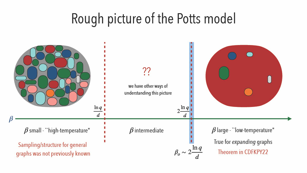
Another result we have is:

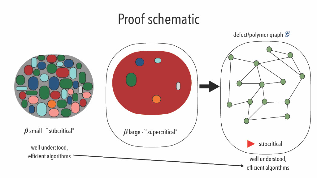
The strategy we have, to prove the theorem for $\beta <(1-𝜖){\beta }_0$:

• Pass to the Random Cluster Model
• Distribution on subsets of edges: $p(A)\propto q^{k(A)}{(e^{\beta }-1)}^{\left|A\right|}$
• $Z_G^{\mathit{RC}}(q,\beta )=Z_G^{\mathit{Potts}}(q,\beta )$
• Sampling algorithm: Sample from random cluster model, give each connected component a uniform color
• Standard polymer methods + careful enumeration

2.8 Polymer Methods

The motivating idea is to visualize the state for $\beta$ large at low temperature as ground state + defects.

Typical Colouring = Ground State + Defects

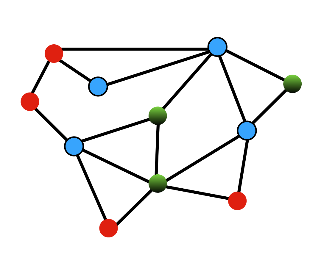
Polymer methods are pretty useful in such cases. These were first proposed in [8] and originated in statistical physics. We take $G$ to be our defect graph and each node in this represents a defect.

Now using Polymer methods $X{\text{∼}}_{G}Y$

Ideas is to $Z_G(q,\beta )\sim Z_{\mathit{red}}+Z_{\mathit{blue}}+\dots$ where $Z_{\mathit{red}}\approx e^{\mathit{\beta nd}∕2}$

$Z_{\mathit{red}}{e}^{-\mathit{\beta nd}∕2}={\sum <!--\; FUNCTION\; APPLICATION\; -->}_{I\subset V(G)}{\prod }_{\gamma \in I}{w}_{\gamma }$ where $w_{\gamma }$ is the weight of polymer $\gamma$.

We now move towards cluster expansion: multivariate in the $w_{\gamma }$ Taylor expansion of:

This is an infinite sum, so convergence is not guaranteed however convergence can be established by verifying the Kotecký-Preiss criterion.

We also want to answer how many connected subsets are there of a given edge boundary in an $\eta$-expander?

A heuristic we have is to count the number of such subsets that contain a given vertex $u$: a typical connected subgraph of size $a$ is tree-like, i.e., has edge boundary $a\cdot d$.

Working backward, a typically connected subgraph with edge boundary size $b$ has $O(b∕d)$ vertices. The number of such subgraphs $\le$ number of connected subgraphs of size $O(b∕d)$ containing $u$. The original number of subsets is also $\le$ Number of rooted (at $u$) trees with $O(b∕d)$ vertices and maximum degree at most $d=d^{O(b∕d)}$. Thus,

Another question to ask is how many $q$-colorings of an $\eta$-expander induce at most $k$ non-monochromatic edges?

Easiest way is to make $k$ non-monochrimatic edges is to color all but $k∕d$ randomly chosen vertices with the same color. Now, $k$ small $\Rightarrow$ these vertices likely form an independent set. we now color these $k∕d$ vertices arbitrarily. There are:

ways.

Now we also know the maximum value of $Z_G(q,\beta )$ over all graphs $G$ with $n$ vertices, $m$ edges, and max degree $d$. This will always be attained when $G$ is a disjoint union of $K_{d+1}$ and $K_1$

3 Statistical Learning using Compression

18th October 2022

The related paper: Adversarially Robust Learning with Tolerance by Ashtiani et al. [9]. Seminar by Hassan Ashtiani.

3.1 Abstract

Characterizing the sample complexity of different machine learning tasks is one of the central questions in statistical learning theory. For example, the classic Vapnik-Chervonenkis theory characterizes the sample complexity of binary classification. Despite this early progress, the sample complexity of many important learning tasks — including density estimation and learning under adversarial perturbations — are not yet resolved. In this talk, we review the less conventional approach of using compression schemes for proving sample complexity upper bounds, with specific applications in learning under adversarial perturbations and learning Gaussian mixture models.

3.2 Some background

We start by defining some notation:

• $Z$: domain set
• $D_Z$: distribution over $Z$
• $S$: i.i.d sample from $D_Z$
• $H$: class of models/hypotheses
• $L(D_Z,H)\to ℝ$: loss/ error function
• $\mathit{OPT}=\mathit{in}{f}_{h\in H}L(D_z,h)$: best achievable
• $A_{Z,H}:Z^{\text{∗}}\to H$: learner

3.3 Density Estimation

Our goal is that for every $D_Z$, $A_{Z,H}(S)$ we want it to be comparable to $\mathit{OPT}$ with high probability.

We take the example of density estimation in this case $L(D_Z,h)=d_{\mathit{TV}}(D_z,h)$. Now, $A_{Z,H}$ probably approximately correct learns $H$ with $m(𝜖,\delta )$ samples if for all $D_Z$ and for all $𝜖$ with a $\delta \in (0,1)$. Now if $S\sim D_Z^{m(𝜖,\delta )}$ then:

Now if we take the example of $C=2$, let $H$ be the set of all Gaussians in ${ℝ}^d$ then:

We will now modify the above equation. Now, $A_{Z,H}$ probably approximately correct learns $H$ with $m(𝜖)$ samples if for all $D_Z$ and for all $𝜖\in (0,1)$. Now if $S\sim D_Z^{m(𝜖)}$ then:

For the example of $C=2$, let $H$ be the set of all Gaussians in ${ℝ}^d$ then:

3.4 Binary Classification (with adv. pertubations)

For the example of binary classification, we have $Z=X\times \{0,1\}$ and $h$ is some model which maps from $h:X\to \{0,1\}$.

We also have $l(h,x,y)=1h(x)\ne y$ and then we will have the $L$ be $L(D_Z,h)=E_{(x,y)\sim D_Z}l(h,x,y)$.

Now, $A_{Z,H}$ probably approximately correct learns $H$ with $m(𝜖)$ samples if for all $D_Z$ and for all $𝜖\in (0,1)$. Now if $S\sim D_Z^{m(𝜖)}$ then:

Now $H$ is the set of all half spaces in ${ℝ}^d$ then:

For the example of binary classification, we have $Z=X\times \{0,1\}$ and $h$ is some model which maps from $h:X\to \{0,1\}$.

We also have $l^U(h,x,y)=$ adversarial pertubations and then we will have the $L^U$ be $L^U(D_Z,h)=E_{(x,y)\sim D_Z}{l}^U(h,x,y)$.

Now, $A_{Z,H}$ probably approximately correct learns $H$ with $m(𝜖)$ samples if for all $D_Z$ and for all $𝜖\in (0,1)$. Now if $S\sim D_Z^{m(𝜖)}$ then:

Now, consider the following $H_1$ and $H_2$:

Here $H_2$ is richer which can make it contain better models as well as harder to learn. We can characterize the sample complexity of learning $H$ using Binary classification, with Binary classification with adversarial perturbations or with Density estimation.

In the case of binary classification the VC-dimension quantifies complexity:

The upper bound here is achieved using simple ERM

And then for uniform convergence:

We now introduce sample compression as an alternative.

3.5 Sample Compression

The idea is to try and answer how should we go about compressing a given training set? In classic information theory, we would compress it into a few bits. In the case of sample compression, we want to try to compress it into a few samples.

If we just take the simple example of linear classification Number of required bits is unbounded (depends on the sample).

It has already been shown by Littlestone and Warmuth [10] that Compressibility $\Rightarrow$ Learnability

It has also been shown by Moran and Yehudayoff [11] Compressibility $\Leftarrow =$ Learnability

Sample Compression can be very helpful by:

• being simpler and more intuitive
• being more generic. It can work even if uniform convergence fails! Can show optimal SVM bound and we can also perform compression for learning under Adversarial Perturbations.

Typical classifiers are often:

• Sensitive to “adversarial” perturbations, even when the noise is “imperceptible”
• Vulnerable to malicious attacks
• Ignore the “invariance” or domain-knowledge

In the case of classification with adversarial perturbations we had $l^{0∕1}(h,x,y)=1\{h(x)\ne y\}$ and $l^U(h,x,y)=\mathit{su}{p}_{\overline{x}\in U(x)}{l}^{0∕1}(h,\overline{x},y)$

and then we will have the $L^U$ be $L^U(D_Z,h)=E_{(x,y)\sim D_Z}{l}^U(h,x,y)$.

Now, $A_{Z,H}$ probably approximately correct learns $H$ with $m(𝜖)$ samples if for all $D_Z$ and for all $𝜖\in (0,1)$. Now if $S\sim D_Z^{m(𝜖)}$ then:

However one of the problems with this is if the robust ERM works for all $H$

The robust ERM would not work for all $H$, uniform convergence can fail,

can be unbounded.

We can say that any “proper learner” (outputs from $H$) can fail.

In a compression-based method the decoder should recover the labels of the training set and their neighbors and then compress the inflates set:

So,

There is an exponential dependence on $VC(H)$.

Ashtiani et al. [9] introduced tolerant adversarial learning $A_{Z,H}$ PAC learns $H$ with $m(𝜖)$ samples

if $\forall <!--\; FUNCTION\; APPLICATION\; -->D_Z$, $\forall <!--\; FUNCTION\; APPLICATION\; -->𝜖\in (0,1)$, if $S\simeq D_Z^{m(𝜖)}$ then

And,

The trick is to avoid compressing an infinite set and now our new goal is that the decoder should only recover labels of things in $U(x)$.

To do so we can define a noisy empirical distribution (using $V(x)$) and then use boosting to achieve a super small error with respect to this distribution. And then, we encode the classifier using the samples used to train weak learners and the decoder smooths out the hypotheses.

It is interesting to think of Why do we need tolerance? There do exist some other ways to relax the problem and avoid $2^{O(VC)}$

• bounded adversary
• Limited black-box query access to the hypothesis
• Related to the certification problem

This is also observable in the density estimation example.

3.6 Gaussian Mixture Models

Gaussian mixture Models are very popular in practice and are one of the most basic universal density approximators. These are also the building blocks for more sophisticated density classes and can think of them as multi-modal versions of Gaussians.

We say $F$ is Gaussian Mixture Model with $k$ components in ${ℝ}^d$. And we want to ask how many samples is needed to recover $f\in F$ within $L_1$ error $𝜖$.

The number of samples $\simeq m(d,k,𝜖)$.

To learn single Gaussian in ${ℝ}^d$ then

samples are sufficient (and necessary).

Now if we have $k$ Gaussian in ${ℝ}^d$ then we want to know if

samples are sufficient?

There have been some results on learning Gaussian Mixture Models.

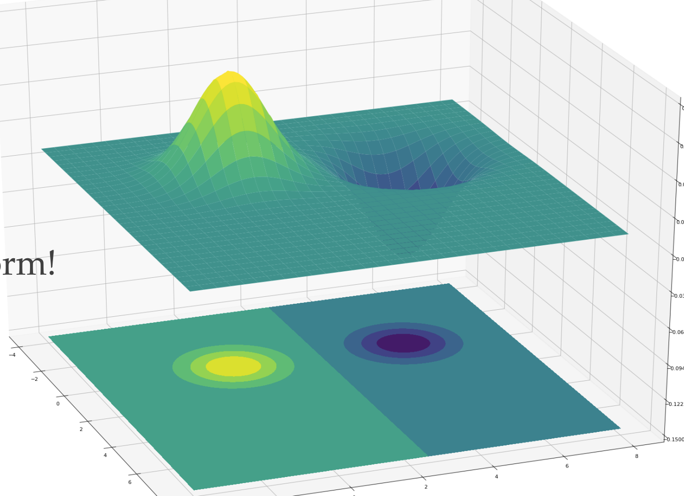
Let us take the example of this graph. For a moment look at this as a binary classification problem. The decision boundary has a simple quadratic form!

Here “Sample compression” does npt make sense as there are no “labels”.

3.7 Compression Framework

We have $F$ which is a class of distributions (e.g. Gaussians) and we have. If A sends $t$ points from $m$ points and B approximates $D$ then we say $F$ admits $(t,m)$-compression.

Small compression schemes imply sample-efficient algorithms.

Distribution compression schemes extend to mixture classes automatically! So for the case of GMMs in ${ℝ}^d$ it is enough to come up with a good compression scheme for a single Gaussian!

For learning mixtures of Gaussians, the encoding center and axes of ellipsoid is sufficient to recover $N(\mu ,\mathrm{\Sigma })$. This admits $Õ(d^2,\frac{1}{𝜖})$ compression! The technical challenge is encoding the $d$ eigenvectors “accurately” using only $d^2$ points.

$\frac{{\sigma }_{\mathit{max}}}{{\sigma }_{\mathit{min}}}$ can be large which is a technical challenge.

3.8 Conclusion

• Compression is simple, intuitive, generic

• Compression relies heavily on a few points

  • But still can give “robust” methods
  • Agnostic sample compression
  • Robust target compression

• Target compression is quite general

  • Reduces the problem to learning from finite classes
  • Does it characterize learning?

References