What is Induction?
Some things I learned from and thought about while taking a philosophy course (my first one!) called Probability and Inductive Logic.
Induction (not to be confused with mathematical induction) is the step that turns finite observations into claims about cases we have not observed, and this article is about why that step is so hard to justify. The data itself does not say how it should be continued, so to make a projection we have to add structure: a language for the hypotheses, a probability space, a class of allowed continuations, some notion of evidence, and some goal like probability raising, convergence, error control, or eventually learning the truth. Most of the article is really about pinning down where exactly that structure ends up sitting in each particular formalism.
The theme running through the article is that induction is a family of projection rules under chosen structure, and the interesting question is to see where the structure enters and what each formalism actually justifies. Most of these rules look very different from each other on the surface, but each one comes down to a choice of representation paired with a rule that turns the representation into a prediction. The hard part of induction is almost never the rule itself, it is the representation that the rule is defined over.
The Basic Problem
The basic pattern is:
\[\text{some things I have observed} \quad \rightsquigarrow \quad \text{some things I have not observed}.\]All observed ravens have been black, so the next raven will probably be black. The wine in this glass is good, so the bottle is probably good. The allergy test is positive, so the allergy is probably present. Usually, a theory predicts an observation, the observation happens, and we say the theory has been confirmed. The question we want to answer is normative: we want to know when the inference from observed cases to unobserved cases may be made, and why.
The simplest form of induction is something like:
\[\text{All observed }F\text{s have been }G.\]Therefore,
\[\text{the next }F\text{ will be }G.\]Or more ambitiously,
\[\text{all }F\text{s are }G.\]The inference is not deductively valid: the premises can all be true while the conclusion is false, since every raven observed so far can be black and the next one can still turn out to be white. A deductive argument cannot give us genuinely new information about unobserved cases unless something about those cases was already built into the premises, which is precisely what inductive arguments try to do, and using induction to justify that move is itself circular.
Hume’s problem is that we want a justification of the rule:
\[\text{past regularity} \quad \Longrightarrow \quad \text{future regularity}.\]If the justification is deductive, it cannot go beyond the evidence. If it is inductive, it presupposes the principle it is supposed to justify. The point is not to stop predicting things, since science and ordinary life both use induction routinely and successfully; the question is what kind of structure has to be added before such a projection counts as reasonable.
Confirmation Needs Background
Prediction is Not Enough
One tempting idea is that evidence confirms a hypothesis exactly when the hypothesis predicts the evidence: if $h$ implies $e$ and $e$ in fact happens, $e$ confirms $h$. There is something right in this, since a hypothesis that makes an observation expected does look better when the observation occurs than one that did not predict anything. But logical implication on its own turns out to be too weak a hook to hang confirmation on.
Suppose $h$ is general relativity and $e$ is the proposition that Mercury has the observed anomalous perihelion advance. If $h$ together with the usual background assumptions implies $e$, then $e$ confirms $h$.
But $h \wedge x$ also implies $e$ for any irrelevant $x$, so the same observation confirms
\[\text{general relativity} \wedge \text{there is life on Mars},\]even though the evidence has no apparent bearing on Mars. Disjunction gives the dual problem: if $h$ implies $e$, then $h$ implies $e \vee x$, so a true but irrelevant disjunction can appear to confirm a hypothesis as well. For example, “Toronto is a city or Muhammad Ali is immortal if he is human” can become evidence for “all humans are immortal” if we read confirmation only through this bare hypothetico-deductive shape.
Logical implication is doing what it is supposed to do here, and the trouble is that confirmation needs more than implication. It needs relevance, background, and some account of the alternatives we are comparing against.
So confirmation is almost never a two-place relation between evidence and hypothesis but a three-place relation
\[e \text{ confirms } h \text{ given } b,\]where $b$ is the relevant background information. Clouds confirm rain only against meteorological background assumptions, a positive allergy test confirms the allergy only against assumptions about the test, and Mercury’s perihelion confirms a theory only against assumptions about observation, calculation, auxiliary physics, and the absence of certain systematic errors.
This background decides which observations are surprising, which alternatives matter, and which implications are evidentially relevant.
The Raven Paradox
The ravens paradox looks artificial at first sight, but it exposes a real problem for purely logical accounts of confirmation. Let
\[h = \forall x(R(x) \to B(x))\]be the hypothesis that all ravens are black. A black raven intuitively seems to confirm $h$, which matches Nicod’s criterion that a universal generalization is confirmed by its positive instances. But $h$ is logically equivalent to
\[\forall x(\neg B(x) \to \neg R(x)),\]the claim that all non-black things are non-ravens.
A green apple is a non-black non-raven and therefore a positive instance of the contrapositive, so if logically equivalent hypotheses are confirmed by the same evidence, a green apple confirms that all ravens are black. At first this seems absurd, since looking at apples is not what we usually call ornithology, but the paradox is not so easy to dismiss. The two hypotheses really are logically equivalent: if evidence supports one proposition, why should it not support an equivalent one, and if positive instances confirm universal generalizations, why should a non-black non-raven not confirm the universal generalization that all non-black things are non-ravens?
One response is to accept the conclusion as stated and treat the confirmation as extremely weak: a green apple does confirm the raven hypothesis, but much less than a black raven does. This is really a limitation of purely qualitative confirmation, since if the only question is
\[\text{does }e\text{ confirm }h?\]the answer can hide important differences, while if we ask the quantitative question
\[\text{how much does }e\text{ confirm }h?\]the result is much easier to interpret. A black raven is much more diagnostic than a green apple, because given any plausible background there are vastly more non-black non-ravens than ravens, so seeing one more green apple barely moves the probability at all.
We can see this in a rough likelihood comparison. Suppose there are $N_R$ ravens and $N_{\neg B}$ non-black objects, with $N_{\neg B}\gg N_R$. If $h$ is false because $k$ ravens are non-black, then sampling a raven and seeing that it is black has likelihood
\[P(B\mid R,h)=1,\]while under $\neg h$ it has likelihood
\[P(B\mid R,\neg h)=1-\frac{k}{N_R}.\]The likelihood ratio is therefore
\[\frac{P(B\mid R,h)}{P(B\mid R,\neg h)} = \frac{1}{1-k/N_R}.\]Now compare this to sampling a non-black object and seeing that it is not a raven. Under $h$, every non-black object is a non-raven:
\[P(\neg R\mid \neg B,h)=1.\]Under $\neg h$, only the $k$ non-black ravens spoil this:
\[P(\neg R\mid \neg B,\neg h)=1-\frac{k}{N_{\neg B}}.\]Since $N_{\neg B}$ is enormous compared with $N_R$, the likelihood ratio for the green apple is much closer to $1$. It confirms in the formal sense, but it is almost non-diagnostic.
The ravens paradox forces the background assumptions into view: without them the formal rule produces counterintuitive consequences, and with them we can explain why the confirmation from a green apple ends up so weak. This does not fully dissolve the paradox, because logical equivalence preserves truth conditions but it does not preserve the usefulness of a description for inquiry. “All ravens are black” and “all non-black things are non-ravens” say literally the same thing, yet they do not suggest the same experiment.
Falsification and Auxiliaries
Falsification seems at first to avoid the problem entirely. If $h \to e$ and we observe $\neg e$, then $\neg h$ follows by modus tollens, which is a deductively valid step, and although finitely many positive instances cannot verify a universal hypothesis, a single counterexample is enough to falsify it: one non-black raven refutes “all ravens are black,” and this asymmetry between universal hypotheses and their instances is one of the main motivations for falsificationism.
But actual tests almost never look like $h \to e$. They usually look more like
\[h \wedge a_1 \wedge a_2 \wedge \cdots \wedge a_n \to e,\]where the $a_i$ are auxiliary assumptions, measurement assumptions, background theory, assumptions about the experimental setup, and so on.
When $\neg e$ happens, all deductive logic actually gives us is
\[\neg(h \wedge a_1 \wedge a_2 \wedge \cdots \wedge a_n),\]i.e. something in the conjunction failed, but the rule does not tell us which conjunct to blame. The failure could lie in the main hypothesis, in an auxiliary theory, in an instrument, in the experimental setup, or even in the derivation itself, and deciding which assumption to discard requires the kind of judgment that modus tollens does not supply on its own. So falsification works reasonably well as a methodological attitude (severe tests and failed predictions both matter), but the actual job of deciding what has been falsified is not done by the logical rule.
A related issue is that many hypotheses we care about are not falsifiable in Popper’s strict sense in the first place. “Every planet will at some point have life on it” is not falsified by observing any finite number of currently lifeless planets, because to falsify it one would need to verify that some particular planet never has life at any time, which is itself a universal claim about an infinite future. So the falsification picture, taken as a clean replacement for inductive reasoning, is too neat: it catches a real asymmetry between universal hypotheses and their instances, but actual hypotheses come embedded in background assumptions that the picture has to either ignore or quietly smuggle in.
Probability Needs a Representation
Probability Spaces
The probabilistic account of confirmation is much more precise. Evidence $e$ incrementally confirms a hypothesis $h$ given background $b$ exactly when
\[P(h \mid e \wedge b) > P(h \mid b),\]i.e. when the evidence raises the probability of the hypothesis. Under regularity assumptions this is equivalent to the likelihood form
\[P(e \mid h \wedge b) > P(e \mid \neg h \wedge b),\]which is often the easier of the two to use, since it says evidence confirms a hypothesis when the evidence is more expected under the hypothesis than under its negation.
This framework already handles several of the difficulties we just met. If $e$ falsifies $h$, then $P(h \mid e \wedge b)=0$ and $e$ disconfirms $h$. If $h \wedge b$ implies $e$ and $b$ alone does not, then $e$ is strictly more expected given $h$ than without it, so successful prediction becomes a special case of probabilistic confirmation. The ravens paradox also looks much better, since a non-black non-raven can confirm that all ravens are black but less than a black raven does, once we include background assumptions like there being many more non-black things than ravens.
The remaining and harder difficulty is where the probability model itself comes from. Before we can write $P(h \mid e)$, we already need a space of possibilities, a language of hypotheses, an algebra of propositions, and a probability measure, and none of those choices is forced on us by the probability calculus.
A probability space is usually written as
\[\langle W,\mathcal A,P\rangle.\]Here $W$ is a non-empty set of possible worlds or outcomes, $\mathcal A$ is an algebra of propositions over $W$, and $P$ assigns probabilities to propositions in $\mathcal A$. A subset of $W$ that is not in $\mathcal A$ has no probability at all, which is a strictly different situation from having probability zero (probability zero is still a perfectly good probability value), so even before assigning any numbers we have already decided which distinctions in $W$ are available to us.
For a coin toss, we might choose
\[W=\{H,T\}.\]Or maybe
\[W=\{H,T,N\},\]where $N$ is some abnormal outcome. For two tosses, we might choose
\[W=\{HH,HT,TH,TT\},\]or we might collapse order and choose
\[W=\{2H,1H1T,2T\}.\]These spaces are not the same. A uniform distribution over the first two-toss space gives different weights to counts than a uniform distribution over the count-space.
In the ordered space,
\[W_1=\{HH,HT,TH,TT\},\]uniformity gives
\[P(HH)=P(HT)=P(TH)=P(TT)=\frac14.\]So the induced probability of exactly one head is
\[P(\text{exactly one }H)=P(HT)+P(TH)=\frac12.\]In the count-space,
\[W_2=\{2H,1H1T,2T\},\]uniformity gives
\[P(2H)=P(1H1T)=P(2T)=\frac13.\]Both choices can be described as “uniform,” but they are uniform over different objects, and the sample space is itself a part of the inductive model. So “assign a probability” really hides two choices: first choosing the space and then assigning weights inside that space — and the first of these is where most of the philosophical problem actually lives.
Uniform Over What?
The classical interpretation of probability says that if cases are equally possible, probability is favorable cases divided by total cases: six equally possible cases for a fair die, two for a coin, and so on. This works as long as we know what “equally possible” actually means, and Bertrand’s chord paradox shows that this is not as simple as it sounds.
Draw a random chord in a circle. What is the probability that the chord is longer than a side of the inscribed equilateral triangle? There are three standard answers.
If we choose two random endpoints on the circumference, the answer is
\[\frac13.\]If we choose a random point on a radius and draw the perpendicular chord, the answer is
\[\frac12.\]If we choose a random midpoint in the disk, the answer is
\[\frac14.\]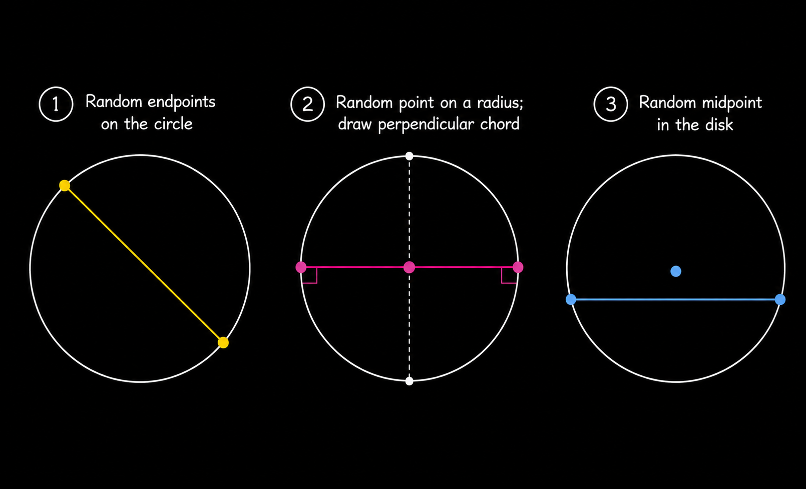
Probability theory is perfectly consistent here; the phrase “random chord” simply did not specify which random experiment we were doing in the first place.
The wine/water paradox makes the same point through reparameterization. Suppose a liquid has wine-to-water ratio $x$ between $1/3$ and $3$. If we treat $x$ as uniformly distributed, we get one answer for
\[P(x\leq 2).\]If we treat the water-to-wine ratio $y=1/x$ as uniformly distributed, we get another. If we treat the proportion of wine $z$ as uniformly distributed, we get a third.
Each of these looks like a representation of ignorance, but the first is biased toward wine, the second toward water, and the third toward neither, so the example makes the underlying assumption explicit: ignorance is not invariant under change of coordinates. The same issue appears for maximum entropy, which says that among probability distributions satisfying the constraints we know, we should pick the one with maximum entropy
\[H(P)=-\sum_i P(w_i)\log P(w_i).\]This gives a principled version of “do not add extra information,” and relative entropy generalizes the same idea by choosing the new distribution that is closest to the old one subject to the new constraint. But the constraints and variables themselves still have to be chosen up front, so MaxEnt is also a rule relative to a chosen representation, not something that floats above all of them.
Conditional Probability
One small distinction that prevents a lot of confusion:
\[P(B\mid C)\]is not, in general,
\[P(C\to B).\]Conditional probability restricts attention to the $C$-cases and asks how often $B$ holds among them, while the material conditional $C \to B$ is true whenever $C$ is false or $B$ is true, so $P(C\to B)$ can be large simply because $C$ is usually false, which tells us almost nothing about whether $B$ is likely given $C$. This matters because ordinary language encourages us to slide between “if $C$, then $B$” and “$B$ given $C$” as if they were the same thing, while in probability theory they are different objects with very different behavior.
There is also the zero-probability issue: if $P(C)=0$ then $P(B\mid C)$ is undefined, because we cannot divide by zero. This matters for confirmation because many standard definitions silently require the evidence and the background to have positive probability, and one alternative is to take conditional probability as primitive and define the ordinary probability as $P(\cdot \mid W)$ instead. That proposal actually sits closer to how probabilities get used in practice, where they are almost always already relative to some background condition.
Projectibility and Model Classes
State and Structure Descriptions
One ambitious thought is that probability might be logical: evidence should support a hypothesis to some specific degree purely as a matter of logic, independently of anyone’s psychology and of any physical chance. To make this precise, we can imagine a formal language with individual constants $a,b,\ldots$ and predicates $F,G,\ldots$.
A state description says completely, for each named individual and each primitive predicate, whether the individual has the predicate. With two individuals $a,b$ and one predicate $F$, the four state descriptions are:
\[F(a)\wedge F(b),\] \[F(a)\wedge \neg F(b),\] \[\neg F(a)\wedge F(b),\] \[\neg F(a)\wedge \neg F(b).\]A structure description forgets the names and remembers only the pattern, so the two middle state descriptions above both belong to the same structure: exactly one of the two individuals is $F$. The structure-description move is to assign equal probability to each structure description and then divide each structure’s total weight uniformly among the states that fall inside it, which gives the structures
\[\text{two }F,\quad \text{one }F,\quad \text{zero }F,\]each with weight $1/3$, and since the middle structure contains two state descriptions, each of those gets $1/6$:
\[P(F(a)\wedge F(b))=\frac13,\] \[P(F(a)\wedge \neg F(b))=\frac16,\] \[P(\neg F(a)\wedge F(b))=\frac16,\] \[P(\neg F(a)\wedge \neg F(b))=\frac13.\]Then observing $F(a)$ raises the probability of $F(b)$:
\[P(F(b)\mid F(a))=\frac23>\frac12.\]In this model, seeing one $F$ already makes another $F$ more likely. If instead we had assigned equal probability to each state description, observing $F(a)$ would not raise the probability of $F(b)$ at all, because the individuals would be too independent of one another to allow any learning from experience to happen.
This example matters because the choice between state descriptions and structure descriptions ends up determining whether the model permits any inductive learning in the first place. Equal-over-states and equal-over-structures are both symmetry principles, but they encode quite different expectations about the world, and the structure-weighted version is the one that builds in a tendency toward uniformity, which is precisely why it supports induction at all.
This generalizes into a whole continuum of inductive rules indexed by a parameter $\lambda \ge 0$,
\[c_\lambda(F(a_{n+1})\mid e_N) = \frac{k+\lambda/\kappa}{N+\lambda},\]where $N$ is the sample size, $k$ is the number of $F$’s observed so far, $\kappa$ is the number of cells of the partition the predicate sits in, and $\lambda$ controls how much weight is given to the logical factor relative to the empirical relative frequency $k/N$. As $\lambda \to 0$ the rule collapses to the straight rule of relative frequencies, and as $\lambda \to \infty$ it collapses to the logical $1/\kappa$ that ignores experience entirely; finite $\lambda$ is what actually mixes the two.
Mathematically this looks like smoothing or pseudo-counts, but maybe we can simply state it as a mixture of experience and logical structure, and the next question is why we should pick any particular mixture at all. One answer appeals to intuitive judgments about inductive validity, but then the justification is no longer purely deductive, and if the underlying inductive principles are supposed to be a priori but not analytic in the sense of being provable, they start to look like synthetic a priori truths, which sits uneasily with the logical empiricism that motivated the project in the first place.
The more interesting point is that inductive structure has to enter somewhere: if it is not in the observed data, it enters through the language, the prior, the weighting of structures, the choice of predicates, or the update rule, and there is no escape from putting it in somewhere, no such thing as a purely formal induction.
Grue and Projectibility
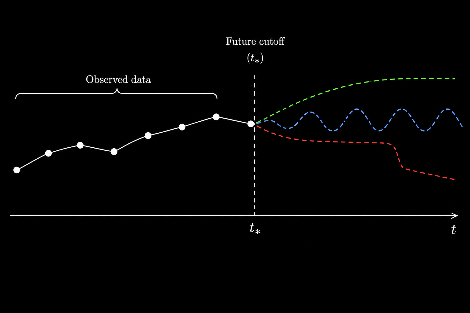
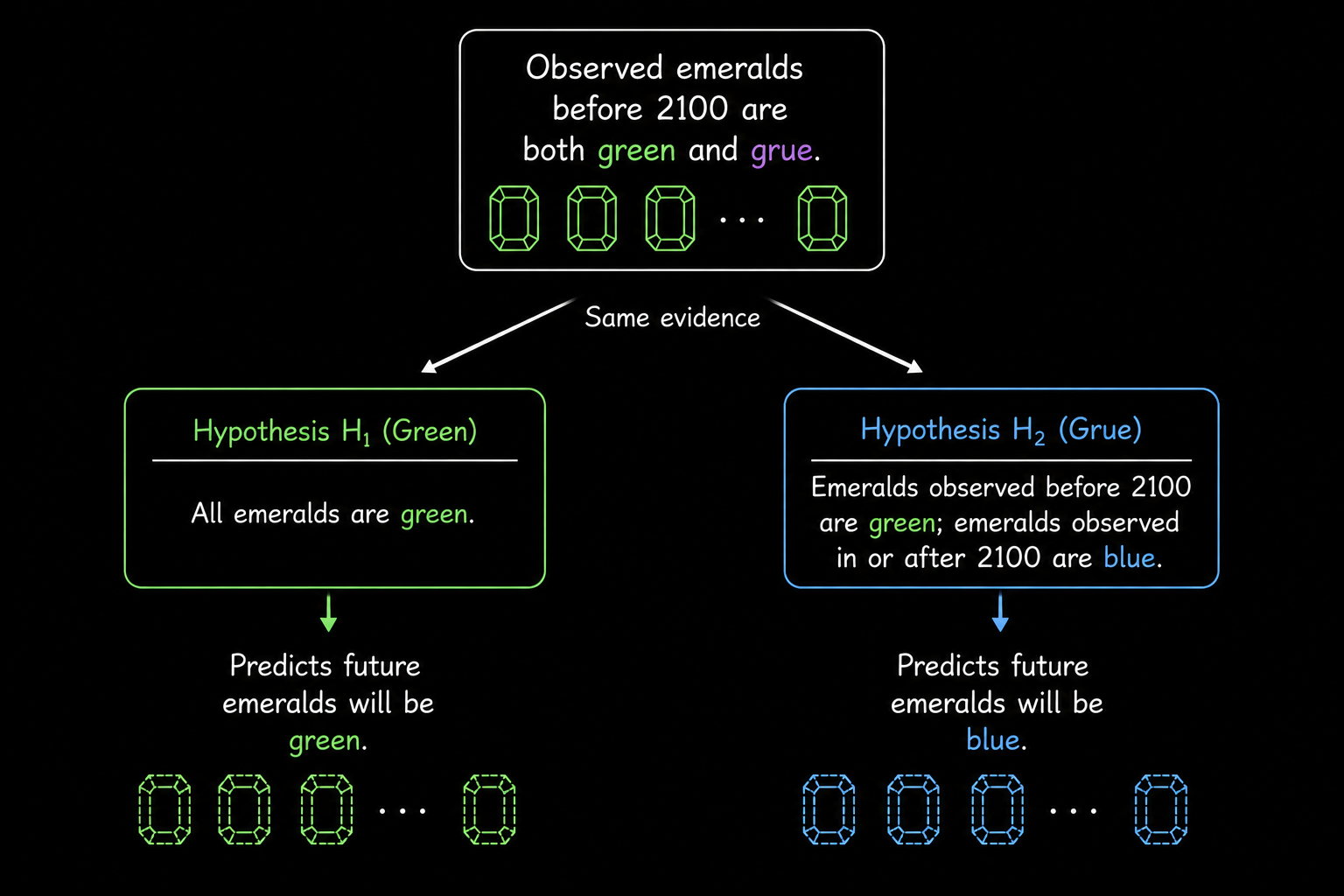
The grue example is also very useful to know about now. Suppose all emeralds observed so far have been green, and we infer that future emeralds will also be green. Now define a new predicate:
\[\text{grue}(x)\]holds iff $x$ is green and observed before January 1, 2100, or blue and observed on or after January 1, 2100. Then every emerald observed so far is green, and every emerald observed so far is also grue, since each was observed before 2100. So why do the observations support
\[\text{future emeralds are green}\]rather than
\[\text{future emeralds are grue}?\]After 2100, a grue emerald is by definition blue, so the two projections disagree as soon as we cross the cutoff.
A common reaction is that “grue” is artificial — but artificial relative to what? If we had instead taken grue and its time-flipped partner bleen (blue before 2100 and green afterwards) as the primitive predicates of our language, then green and blue would be the gerrymandered, time-conditional ones, and the symmetry between the two pairs would look the other way around.
The relevant question is therefore projectibility: which predicates are legitimate for induction in the first place? The finite evidence is compatible with many future continuations and does not, on its own, say which respects of similarity matter. Unobserved objects always resemble observed objects in some respects and fail to resemble them in others; both halves of that observation are trivial, and the real question is
\[\text{which respects of similarity are projectible?}\]Pure syntax does not answer this, and neither does pure positive-instance counting.
One answer uses entrenchment: a predicate counts as projectible if it has been used frequently in past successful projections, so “green” is entrenched and “grue” is not. As a description of our actual practice this is reasonable enough and it explains what we do, but normatively it leaves the central question open, because if induction is supposed to tell us what we ought to project, then “project what we have projected” comes dangerously close to deriving an ought from an is.
The riddle therefore changes the question from “how many positive instances are enough?” to “which descriptions of the instances are the right ones to project in the first place?” and a purely logical theory of confirmation simply does not supply that distinction, because it cannot see any difference between green and grue.
Inductive Bias and Model Classes
A similar pattern appears in learning algorithms. Suppose we observe finitely many input-output pairs:
\[D=\{(x_i,y_i)\}_{i=1}^n.\]There are infinitely many functions $f$ such that
\[f(x_i)=y_i\]for every observed point. If the only constraint is interpolation, the data do not determine what $f$ should do at a new point $x_{n+1}$. We need a hypothesis class,
\[\mathcal H=\{h:X\to Y\},\]and usually some preference inside that class:
\[\hat h=\arg\min_{h\in\mathcal H}\sum_{i=1}^n \ell(h(x_i),y_i)+\lambda\Omega(h).\]The hypothesis class $\mathcal H$, the loss $\ell$, and the regularizer $\Omega$ together do exactly the work that “projectibility” does in the grue example: they say which continuations are even allowed, and among those which ones are preferred. A polynomial interpolant, a kernel method with a small RKHS norm, a decision tree of bounded depth, and a convolutional neural network can all fit the observed data exactly and disagree on almost everything else, and the difference between them does not live in the finite dataL it lives entirely in the representation and inductive bias each one carries.
Thus the problem of induction is close to generalization theory. Finite training error is a statement about observed samples. Generalization requires assumptions about the data-generating process, the hypothesis class, the sampling procedure, or the algorithm. It also seems different frameworks formalize different ways in which a continuation is allowed to count as natural.
Belief, Updating, and Action
Belief as Probability
Another route is to interpret probabilities as degrees of belief: on this view a probability function is just an ideal agent’s credence function, and the thesis of probabilism says that rational degrees of belief should obey the probability calculus. The classical argument for this is the Dutch book argument.
Suppose my degree of belief in $A$ is represented by the price I regard as fair for a bet that pays $1$ if $A$ is true and $0$ otherwise. If my prices violate the probability axioms, someone can arrange bets against me so that I lose money no matter what happens.
For example, if $A$ and $B$ are mutually exclusive, additivity requires:
\[P(A\vee B)=P(A)+P(B).\]If my fair price for $A\vee B$ is not the sum of my fair prices for $A$ and $B$, someone can buy and sell the corresponding bets against me in a way that guarantees loss.
The argument supports coherence, but it has an important limitation: betting behavior is not the same thing as belief. It depends on utility, risk attitudes, the value of money, whether I enjoy gambling, and whether the proposition itself matters to me, so I may refuse a million-dollar fair bet because the downside would ruin me, take a bad casino bet because gambling is fun, or price a bet strangely because the truth of the proposition would itself be good or bad for me independently of the payout.
The depragmatized Dutch book argument replaces “willing to bet” with “considers the bet fair,” which helps with this, but now we need a separate argument that fair betting ratios really are degrees of belief. Ramsey’s move is to use utility rather than money, but then we need utility itself to behave nicely. One dollar plus one dollar is two dollars, while the utility of one right shoe plus another right shoe is nowhere near the utility of a usable pair of shoes.
The gradational accuracy argument is closer to a directly epistemic story. A full belief is accurate when it is true, and a partial belief is accurate to the extent that it is close to the truth value of the proposition: $1$ if $A$ is true and $0$ if it is false, so a credence $b(A)$ is inaccurate insofar as it sits far from that truth value.
For a finite partition ${A_1,\ldots,A_n}$, the Brier score is one natural measure:
\[I(b,w)=\frac{1}{n}\sum_i (b(A_i)-w(A_i))^2.\]A belief function is accuracy dominated if there is another belief function that is at least as accurate in every possible world and more accurate in at least one.
The striking theorem is that, under certain assumptions about inaccuracy, the non-dominated belief functions are exactly the probabilistic ones.
This has a quite different flavor from the Dutch book setup, since the claim is that incoherent credences are avoidably worse as estimates of the truth, not that they get punished by a clever bettor. But even taken at its strongest, the accuracy argument still gives only coherence and not correctness: a probabilistic credence function can be coherent and badly calibrated, coherent and based on a terrible prior, or coherent and defined over the wrong partition, so the probability axioms constrain belief without choosing the right way to carve up the world for it to range over.
Confirmation as Probability Raising
Once probabilities are degrees of belief, Bayesian confirmation theory becomes natural.
Evidence $e$ incrementally confirms $h$ given $b$ iff:
\[P(h \mid e\wedge b)>P(h\mid b).\]We can write the same condition several ways:
\[P(h\wedge e\mid b)>P(h\mid b)P(e\mid b),\] \[P(e\mid h\wedge b)>P(e\mid \neg h\wedge b),\] \[P(e\mid h\wedge b)>P(e\mid b).\]There are also different measures of how much confirmation occurs:
\[D=P(h\mid e,b)-P(h\mid b),\] \[R=\frac{P(h\mid e,b)}{P(h\mid b)},\] \[L=\frac{P(e\mid h,b)}{P(e\mid \neg h,b)},\] \[S=P(h\mid e,b)-P(h\mid \neg e,b).\]These measures can disagree about comparative strength while agreeing on the posterior probabilities, which suggests that “amount of confirmation” is not really a single primitive quantity but different measures are asking slightly different questions about the same posterior. Beyond the choice of measure, two more serious conceptual issues remain.
The first is old evidence. If $e$ is already known, then $P(e\mid b)=1$ and therefore $P(h\mid e,b)=P(h\mid b)$, so on the strict probability-raising criterion already-known evidence cannot raise the probability of anything. But old evidence often does seem to confirm new theories: Mercury’s anomalous perihelion advance was already well known before general relativity, and when GTR explained it that looked like a major confirmation of the theory. The problem is that explanation can arrive after the data, and a new theory can reorganize old facts, make them less accidental, derive them from fewer assumptions, and connect them to facts that were previously unrelated, none of which strict conditionalization on an already-known proposition can capture.
The second issue is that Bayesian confirmation does not completely remove irrelevance problems either. If $i$ is independent of $h$ and also of $h\wedge e$, then $e$ can still incrementally confirm $h\wedge i$ whenever it confirms $h$, so Bayesianism improves on the purely deductive hypothetico-deductive picture while leaving relevance somewhat subtle. The formalism is still useful, because it at least locates the remaining assumptions explicitly even when it does not resolve them.
Updating at the Right Grain
Strict conditionalization says that when I become certain of $E$, my new probability for $H$ should be:
\[P^*(H)=P(H\mid E).\]People often describe this as zooming in on the $E$-worlds, but the evidence has to be represented at the right grain for the rule to work as intended. Suppose a die is rolled and I am told it landed $4$. I thereby also learn that it landed even, but I should condition on ${4}$ rather than only on ${2,4,6}$ because although both propositions become certain after the announcement, only one of them is the strongest proposition I actually learned, and updating on a weaker consequence quietly throws away information that the rule itself does not flag.
Jeffrey conditionalization handles cases where experience changes probabilities without making us certain of one proposition. Suppose ${E_1,\ldots,E_n}$ is the most fine-grained partition directly affected by the experience. Then:
\[P^*(H)=\sum_i P(H\mid E_i)P^*(E_i).\]The conditional probabilities inside the cells are held fixed; only the weights of the cells themselves change.
This treats evidence as more flexible than learning a single proposition with full certainty, which fits how perception, testimony, measurement, memory, and inference usually behave: each of them shifts probabilities without producing certainty about any one cell. As before, the formula does not pick its own partition for us; we still have to say which propositions were directly affected by the experience, and the update rule is exact only once the evidential event has been described at the right level of grain.
Actions and Evidence
Decision theory adds utility on top of belief, and the usual rule is to maximize expected utility:
\[EU(a)=\sum_s u(a,s)P(s).\]Expected utility is straightforward when the states are independent of the acts, since taking an umbrella does not affect whether it actually rains, so if I know the probability of rain and the utilities of each outcome, I can simply choose the act with higher expected utility. But many acts of interest are not independent of states at all: studying changes the probability of passing, taking medicine changes the probability of recovery, and exercising changes the probability of future health, all in ways that the simple formula above is not equipped to handle on its own.
Evidential decision theory handles this by using $P(s\mid a)$ in place of $P(s)$, i.e. by asking what the act itself would be evidence for. This works well in the studying case: if
\[P(\text{pass}\mid \text{study})=0.9\]and
\[P(\text{pass}\mid \text{not study})=0.2,\]then studying can have much higher expected utility even if passing without studying would be the best outcome.
Newcomb’s problem creates a difficulty for this whole way of setting things up. There are two boxes: a transparent one containing a thousand dollars, and an opaque one containing either a million dollars or nothing. A predictor that has been almost always correct in the past has already predicted whether I will take only the opaque box or both, and the opaque box contains the million exactly when the predictor predicted one-boxing.
Evidential decision theory recommends one-boxing, because one-boxing is strong evidence that the predictor predicted one-boxing, which is in turn strong evidence that the opaque box contains the million. Causal decision theory recommends two-boxing, because the prediction has already been made and my current action does not causally affect what is already in the box, so whatever is in the opaque box, taking both boxes gives a thousand dollars more than taking the opaque one alone.
The dispute here is conceptual rather than arithmetic: the question is whether rational action should track evidential correlation or causal efficacy. The distinction matters in lots of places that look much more ordinary than Newcomb: a symptom can be evidence of a disease without causing it, a treatment can be correlated with worse outcomes because sicker patients are the ones who receive it even when the treatment in fact helps, and a choice can reveal information about the world without changing the relevant part of the world at all. In other words, conditioning on an action and intervening with an action are simply not the same operation, and any decision theory has to pick which one it is computing with.
Chance, Frequency, and Statistics
Chance and Credence
Chance is another kind of probability-like quantity, and it is worth keeping separate from credence. A subjective probability lives in my state of mind, whereas a chance, at least on realist accounts, lives out in the world, and we infer chances indirectly through theory and observation rather than reading them off directly.
Consider tennis. Before a match starts, there may be some chance that a player begins with an ace, but once the first serve has actually happened, the chance of that event is either $1$ or $0$ — if it happened it happened, and if it did not it did not — while my credence can still be anywhere between $0$ and $1$ as long as I have not yet checked. So chance and credence come apart in a clean way:
\[\text{chance concerns the event relative to the world},\] \[\text{credence concerns the event relative to my information}.\]One slogan for this is:
\[\text{what is past is no longer chancy}.\]The past may be unknown to me, but it is not unsettled in the same way.
Different accounts disagree about what chances really are. One view treats them as propensities, i.e. tendencies of physical setups to produce particular outcomes, while another treats them as whatever the best total theory of the world says they are: on this best-system view, chances belong to the system that best balances simplicity, informativeness, and fit with the actual pattern of events.
The bridge between chance and credence is the Principal Principle:
\[P(A\mid ch_t(A)=x \wedge B_t)=x,\]where $B_t$ is admissible information. If I know the chance of $A$ at time $t$ is $x$, and I have no inadmissible information about whether $A$ in fact occurs, then my credence in $A$ should also be $x$.
The word “admissible” is carrying real weight here, because if I know the chance of heads before a coin toss was $1/2$ but I have already seen that the coin landed tails, I should obviously not assign credence $1/2$ to heads anymore; outcome information is inadmissible in that setting, and the Principal Principle only links chance and credence when no such information has slipped through.
This matters for statistical hypotheses. Suppose we have hypotheses:
\[H_k: ch(E)=\frac{k}{100}\]for $k=0,\ldots,100$, where $E$ is the next toss landing heads.
If we observe heads, it is tempting to write:
\[P(E\mid H_k)=\frac{k}{100}.\]But this is not a theorem of probability. $H_k$ specifies a chance while $P(E\mid H_k)$ is a subjective probability, and substituting one for the other requires a bridge principle saying that a known chance should guide rational credence. Once we have that bridge in place, observing heads confirms the chance hypotheses with $k>50$, but the step is not automatic and it leans entirely on the extra assumption that ties chance to credence.
Reflection is a similar principle about future belief:
\[P_t(A\mid P_{t'}(A)=r)=r.\]If I know that my future credence in $A$ will be $r$, and I do not expect irrationality or misleading evidence in between, then my current conditional credence should already be $r$ as well. The Principal Principle treats chance itself as an expert, while Reflection treats my future self as an expert, and both principles are really screening-off principles: once the expert information is known, no further admissible information should move the probability again.
Convergence Instead of Truth
If we return to Hume’s problem, induction cannot be justified as a rule that always carries true premises into true conclusions, because that demand is far too strong for any rule that goes beyond the data to meet. So the natural move is to change the target of justification.
Consider a sequence of event tokens and an event type $A$. The relative frequency after $n$ observations is:
\[\frac{m}{n},\]where $m$ of the first $n$ events are of type $A$.
The straight rule says: conjecture that the limiting relative frequency is the observed relative frequency,
\[\frac{m}{n}.\]If a coin lands heads twice in three tosses, conjecture that the limiting relative frequency of heads is $2/3$.
At first this rule looks weak, because the conjecture is plainly not guaranteed to be correct at any finite time. The justification is of a different kind:
\[\text{the straight rule converges to the true limiting frequency iff some rule does}.\]If a limiting relative frequency exists, the observed frequency converges to it, and if no such limit exists then there is nothing for any rule of this kind to converge to in the first place.
So the straight rule is vindicated with respect to convergence rather than immediate truth, and the response has a quite different shape from the usual one: it is a deductive argument that a certain inductive rule serves a weaker cognitive end, with an instrumental conclusion,
\[\text{If you want convergence when convergence is possible, use this kind of rule.}\]The circularity charge from Hume plays out differently against this argument, because the argument is about means and ends rather than about premises and conclusions, so the rule is being justified relative to a goal rather than being defended as a guaranteed truth-preserver.
There are two obvious objections to this. The first is Keynes’s line, “in the long run we are all dead,” which says that convergence is too weak a norm to be worth defending in the first place. But many norms in inquiry are structural in this same way: consistency does not guarantee true beliefs either, yet it is still a condition for ever having all true beliefs, and convergence plays a similar role here, since a sequence of conjectures cannot get arbitrarily close to the truth unless it converges to something.
The second objection is that the straight rule is not unique, because a rule that conjectures
\[\frac{m+17}{n}\]also converges to the same limit (since $17/n\to 0$), so the convergence argument by itself does not single out the straight rule. But this only shows that several rules are functionally equivalent relative to the bare end of convergence, and if we care about speed of convergence or finite-sample behavior, we need a more specific end to break the tie.
The same distinction appears in algorithms. Two procedures can have the same asymptotic guarantee and still behave very differently at realistic sample sizes. If the first ten observations contain seven heads, the straight rule outputs $7/10$. A smoothed rule might output
\[\frac{7+\alpha}{10+2\alpha}\]for some pseudo-count $\alpha$. Both can converge to the same limiting frequency, but they make quite different finite-sample predictions, and so convergence is just one norm among several: regret, sample complexity, calibration, and robustness are different norms that the same rule can satisfy or violate independently.
The reference class problem points at a different target altogether.
Suppose I am about to toss a coin. I know this coin landed heads once before. I also know that coins with the same weight landed heads $40\%$ of the time in 20,000 tosses, and coins from the same factory landed heads $60\%$ of the time in 10,000 tosses.
Which reference class should I use?
This exact coin? Coins of the same weight? Coins from the same factory? All coins? Coins tossed in this room?
The narrowest reference class is useless because the exact event is essentially unique, the broadest is too heterogeneous to support any prediction at all, and the middle choices all look arbitrary in different ways. The vindication of the straight rule does not solve this either, because it is a result about convergence in infinite sequences rather than a general method for assigning probabilities to single cases, and the distinction matters: a theorem can solve one problem cleanly and leave a nearby problem completely untouched.
Random Variables and Frequencies
A random variable is neither random nor a variable. It is a measurable function:
\[X:W\to V.\]It maps possible worlds to values. For every measurable set $B\subseteq V$, the inverse image
\[X^{-1}(B)=\{w\in W:X(w)\in B\}\]must be a proposition in the algebra over $W$.
This lets us write things like
\[P(X\in B)\]as shorthand for
\[P(X^{-1}(B)).\]Several random variables generate an algebra of propositions about their values, and if they are independent and identically distributed we are in the familiar iid setting. The Strong Law of Large Numbers says that iid sample means converge almost surely to expected values, so for finite outcome spaces this gives a direct link between probability and frequency: under iid assumptions, relative frequencies converge to probabilities with probability $1$, and if those probabilities are themselves chances, then chance $1$ gets assigned to the proposition that relative frequencies converge to chances.
This lets Bayesian updating over chance hypotheses actually make contact with observed frequencies, since if the true chance hypothesis is in our hypothesis space and has positive prior probability, the trials are iid, and the evidence supplies true relative frequencies, then continuing observations eventually favor the true chance hypothesis. The assumptions are doing serious work in this argument, but inside them chance, frequency, and credence really do line up.
Statistics and Possible Samples
The conceptual issue in statistics is really where probability is placed in the setup. A frequentist confidence interval does not mean
\[P(\mu\in [a,b])=0.95\]for the particular interval after the data have been observed, because the parameter $\mu$ is fixed and the interval is produced by a random sampling procedure, so a $95\%$ confidence procedure is just one that produces intervals containing the true parameter in $95\%$ of repeated samples. It is tempting to read the interval in the Bayesian way, but that would require a probability distribution over $\mu$, while frequentist statistics gives only a probability distribution over possible data or statistics conditional on a hypothesis.
Hypothesis testing has the same structure: we choose a null hypothesis specific enough to assign probabilities to possible sample outcomes, and if the observed sample is sufficiently improbable under the null, we reject it. A Type I error is rejecting a true null, a Type II error is failing to reject a false null, the significance level controls the probability of Type I error, and the power controls the probability of rejecting under a specified alternative.
The interesting wrinkle is that significance can depend on possible samples that were never even observed.
Suppose a device prints zeros and ones. Under the null, each is independent with probability $1/2$. If I decide in advance to observe four bits, then the possible outcomes are all length-four sequences. Under one significance rule, only $0000$ and $1111$ might be extreme enough to reject.
But if I instead decide to observe up to three bits and stop at the first $0$, the possible outcomes are:
\[0,\quad 10,\quad 110,\quad 111.\]Now the evidential status of observing $111$ changes because the sampling plan changed.
The same point appears in optional stopping. Suppose I report a run of heads after checking the data repeatedly and stopping when the result happens to look impressive. The probability of the final string alone is not the whole calculation, because the procedure also made many other impressive-looking strings possible by giving me repeated chances to stop, and a frequentist test evaluates the procedure rather than just the realized sample. The relevant probability is therefore taken over all samples that could have been produced by that procedure, not only over the one sample that ended up being printed in the paper, so the actual data are the same but their significance depends on what might have happened and on when I would have stopped.
The likelihoodist objection is that the evidence should depend only on the probability of the actual data under the hypotheses, not on unobserved possible outcomes; whether that objection fully succeeds is a separate question, but it exposes a real philosophical difference, since frequentist tests are by design about the procedure that generated the data, including the data that could have appeared.
A Bayesian statistician puts probabilities on hypotheses too, so priors over hypotheses combined with likelihoods produce posteriors over hypotheses, while a frequentist usually puts probabilities only on data conditional on hypotheses and never on the hypotheses themselves. Neither side is simply “using probability” while the other is not; they are placing probability in genuinely different parts of the inferential setup.
Learning in the Limit
Formal learning theory gives a quite different way to think about induction: instead of asking for a probability of a hypothesis, we ask whether a method reliably arrives at the correct answer in the long run.
Let an infinite data stream be:
\[\varepsilon=e_1,e_2,e_3,\ldots\]An inductive method sees finite initial segments and outputs hypotheses:
\[\delta(e_1,\ldots,e_n)=H_n.\]The method learns the correct answer if there is some finite time $N$ such that after $N$, it always gives the correct answer:
\[\exists N\ \forall n\geq N:\delta(e_1,\ldots,e_n)=H^*.\]The learner need not know when $N$ has arrived, which is the key move: the framework separates being right eventually from knowing that one is right.
Within this picture, questions split into several quite different classes. Some questions are decidable, in the sense that finite evidence can settle them either way, like “is the third observed raven black?”, which is decidable as soon as the third relevant observation occurs. Some are merely verifiable, where finite evidence can settle yes but never no: “will there ever be a black raven?” gets settled positively as soon as one is observed, and otherwise stays open indefinitely. Some are falsifiable in the dual sense, where finite evidence can settle no but never yes: “are all ravens black?” gets settled negatively by a single non-black raven, and any finite collection of black ravens leaves the universal claim open. Finally, some questions are neither verifiable nor falsifiable at finite time but are still learnable by stabilization, in the sense that a method can eventually settle into the correct answer without any finite sign announcing that it has done so.
This changes the question. Instead of asking:
\[\text{can I know now that I am right?}\]we ask:
\[\text{is there a method that eventually stabilizes on the truth?}\]This is a strictly weaker criterion than knowing at a finite time that one is right, but it still captures a real notion of learning that the strong criterion cannot.
A standard argument against probabilistic inductive logic fits very naturally into this frame: under certain assumptions, no probability measure satisfies an adequacy condition for eventually accepting every true effective hypothesis, while a non-probabilistic method can do exactly that. The caveat is that the argument assumes a computability condition on the probability measure, which not every Bayesian is willing to grant, so the result is not as clean a refutation as it first looks. The learning-theoretic conclusion is nonetheless simple, namely that if a method prevents us from learning things that can be learned, then the method is defective for that particular problem, and the right question to ask of an inductive method is therefore what kind of success is even possible for the problem at hand.
Projection Under Structure
After working through all of these arguments, I have come around to thinking that induction is best treated as a family of projection rules for extending information beyond its original domain, where each rule needs both a background structure and some end by which its success is judged. The background structure can sit in the choice of probability space, the prior, the set of admissible hypotheses, the partition that updating is allowed to act on, the sampling plan, the reference class, or the hypothesis class of a learner, but it always has to sit somewhere, and the substantive content of any inductive method really lies in where it puts that structure rather than in the rule that operates on top of it.
It also seems interesting that evidence is always evidence under a description. The same object can be a black raven, a non-white bird, a non-green non-apple, or a grue emerald, the same sequence of bits can have very different significance under different stopping rules, and the same frequency can either matter or fail to matter depending on which reference class we decide to use. To say what an inductive inference is, we have to say what structure is being projected under, and to defend an inductive inference, we end up having to defend that choice of structure as much as the rule we run on top of it.
Citation
Please cite this work as:
Rishit Dagli. "What is Induction?". Rishit Dagli's Blog (May 2026). https://rishit-dagli.github.io/2026/05/16/induction.htmlOr use the BibTex citation:
@article{ dagli2026what,
  title = { What is Induction? },
  author = { Rishit Dagli },
  journal = {rishit-dagli.github.io},
  year = { 2026 },
  month = { May },
  url = "https://rishit-dagli.github.io/2026/05/16/induction.html"
}