Some of this is actually what I learned in as well as notes from a nice geometry course at the University of Toronto.

Motion has a shape. This article looks at simulation through lens of geometry. If you prefer a computational entry point, skim my simulation primer article first, it complements this view from the Lagrangian side. This article and the simulation primer are closely related, and many of the things I show here clearly fit into the Lagrangian view, the previous article talks about the Lagrangian view. I do recommend reading it first and then coming back here to get many aha moments of just how well things fit in.

This article is mainly focused on the Hamiltonian view to simulation. The Hamiltonian is a very powerful mathematical tool that can represent the main kind of simulations we care about i.e. motion of particles following Newtonian mechanics. However, the Hamiltonian can easily be extended to represent many other kinds of systems, magnetism, and relativity (we only talk a little bit about relativity at the end) all within the same framework! It might seem that it takes a while to buid the overall framework, but once we build it we can easily incorporate many other kinds of systems into the same framework. Another side effect is a lot of Hamiltonian mechanics falls out by taking insights from geometry and overall most of the main ideas are fairly intuitive.

Unlike the previous article, this article requires some more pre-requisites. This article assumes some basic knowledge of differential geometry. But I think this should in general not make the article less accessible because all of the things we assume are popular terms ¹.

Hamiltonian Dynamics

Let us begin with a smooth manifold $X$ which we will call the configuration space. An example is the spring-mass system $X = (\mathbb{R}, q)$.

An example of a simple configuration.

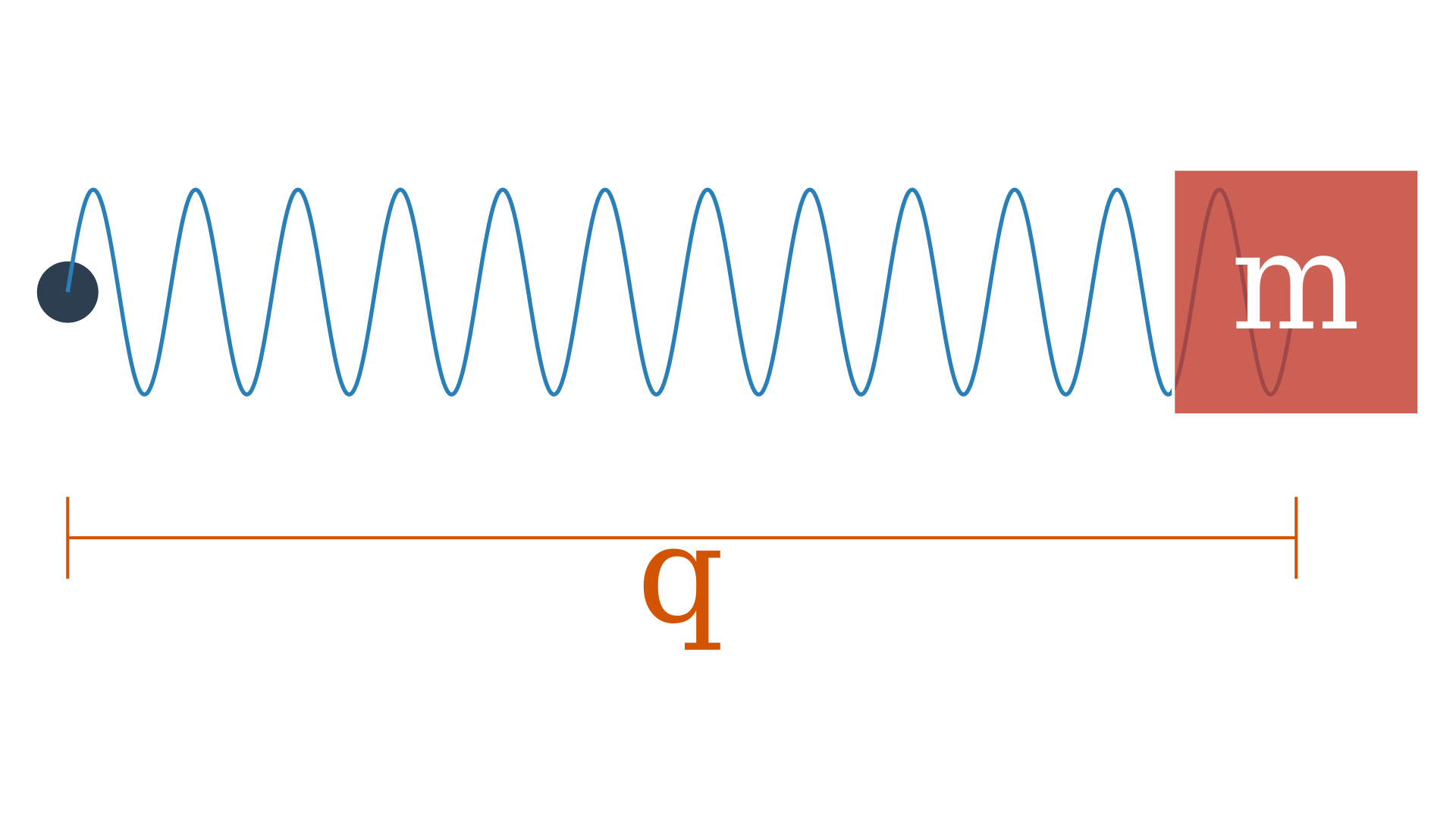
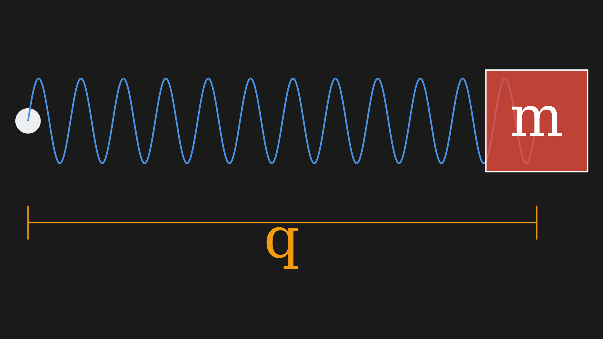
The position of the mass is a configuration which forms a smooth manifold in one dimension. We could also have this in multiple dimensions, $X = (\mathbb{R}^n, (q_1, q_2, \ldots, q_n))$ or the set of complex numbers with norm one $X = S^1 = \lbrace z \in \mathbb{C} : \mid z \mid = 1 \rbrace $ or the $n$-sphere inside the $n+1$-dimensional space $X = S^n \in \mathbb{R}^{n+1} \quad S^n = \lbrace (q^0, q^1, \ldots, q^n) \in \mathbb{R}^{n+1} : \sum_{i=0}^n (q^i)^2 = 1 \rbrace $. These configurations are like point particles moving on a smooth manifold.

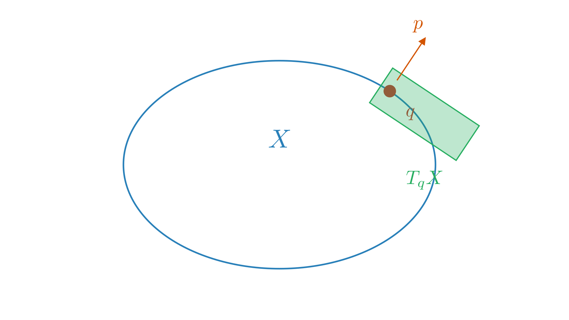
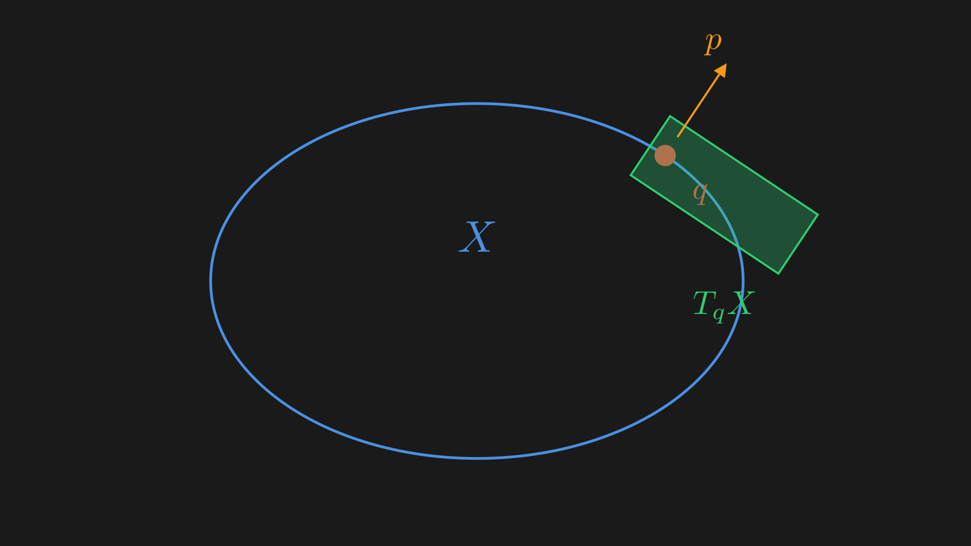
Broadly speaking, the entire purpose of Hamiltonian mechanics is to predict the future or past of a system based on the current state of the system, so, if we fully know some initial state of the system and we know the law it satisfies, we can predict the future or the past. Generally speaking, the future is not just defined by the current “position” or configuration but rather it is uniquely determined by the state of the system. This state consists of $q$: the position and $p$: the momentum. This state is an element of the set which is the cotangent bundle $T^*X$ (the state space or phase space), $(q, p) \in T^*X$. This cotangent bundle is essentially the set of all possible states of the system, $q \in X$, and $p$ is an element in the dual space of the tangent space to $X$ at $q$ and $p \in T_q^*X$. The momentum $p$ is a covector at $q$. This essentially tells us how much momentum there is in a direction $v \in T_qX$.

Momentum is a covector at the point $q$.

A tangent vector at $q \in X$ can be written as,

\begin{equation} v = \overbrace{v^1}^{\text{components}} \underbrace{\frac{\partial}{\partial q^1}}_{\text{vector field}} + \overbrace{v^2}^{\in \mathbb{R}^n} \frac{\partial}{\partial q^2} + \cdots + v^n \frac{\partial}{\partial q^n}. \label{eq:tangent-vector} \end{equation}

The $\frac{\partial}{\partial q^i}$ represents the vector fields that live in the $n$-dimensional space and point in the $q^i$ direction.

A cotangent vector at $q \in X$ can be written as,

\begin{equation} p = \overbrace{p_1}^{\text{components}} \underbrace{dq^1}_{\text{dual basis}} + p_2 dq^2 + \cdots + p_n dq^n. \label{eq:cotangent-vector} \end{equation}

And since it is a dual basis evaluating the vector field $\frac{\partial}{\partial q^i}$ at $dq^i$ gives us $1$ and at any other $dq^j$ gives us $0$. Essentially, by choosing the coordinates $(q^1, q^2, \ldots, q^n)$ we automatically obtain coordinates $(q^1, q^2, \ldots, q^n, p_1, p_2, \ldots, p_n)$ for $T^*X$ (cotangent bundle) which is a $2n$-dimensional smooth manifold. The $(p_1, p_2, \ldots, p_n)$ are called the canonical conjugate variables of $(q^1, q^2, \ldots, q^n)$.

(Main Idea). The evolution in time of the state $(q, p) \in T^*X$ is the flow of a vector field on $T^*X$.

This means if $X=S^1$ then the cotangent bundle of $S^1$, $T^*S^1$ contains a bunch of vector spaces, one for every point on $S^1$. This is because we know for every point on $S^1$ there is a tangent space which is a line or 1-dimensional space and the dual space to that is 1-dimensional space. The $T^*S^1$ is $S^1 \times \mathbb{R}$, which is a cylinder.

The cotangent bundle of $S^1$ is a cylinder.

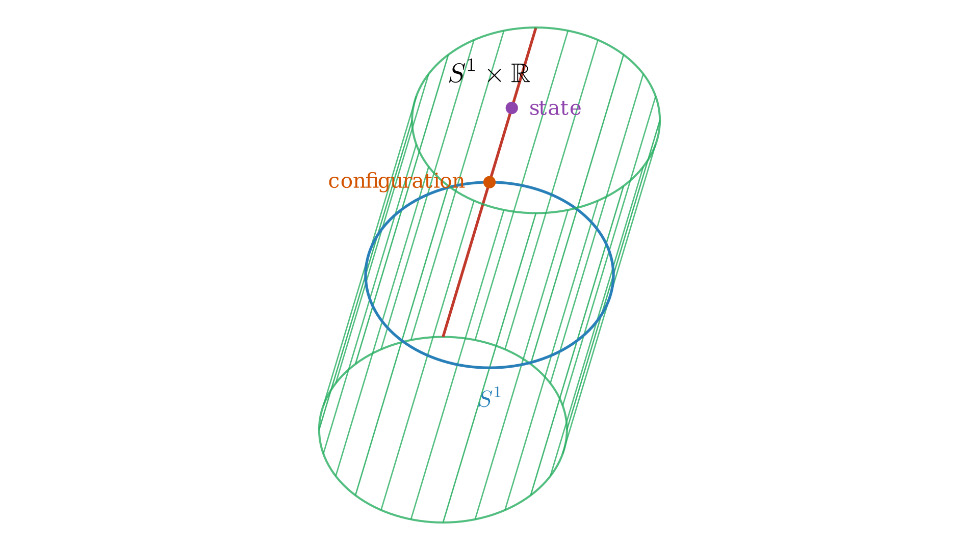
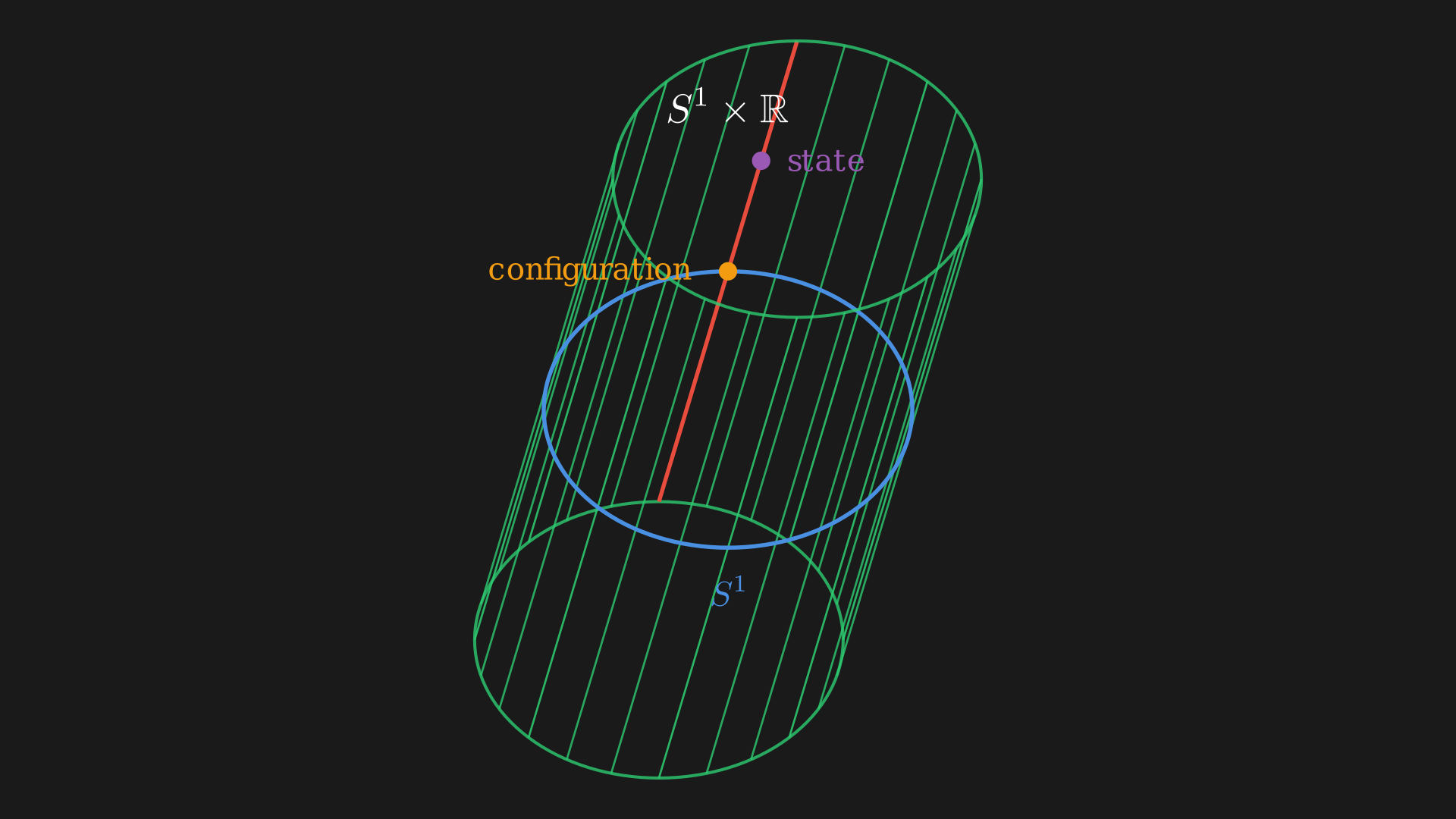
Every point on this cylinder is a state, and to analyze this state we can apply the projection map ² $\pi: T^*X \mapsto X, \pi: (q, p) \mapsto q$ which would map it down to the base space $S^1$ which is in the configuration space. At this point we have a cotangent fiber which is a $1$-dimensional vector space with the origin at the circle or the “zero momentum”. As we go up, we have non-zero momentum. Every possible configuration and every possible velocity is represented in this cotangent bundle.

What this means is to specify the model of this state space all we need to do is provide a vector field on the space of states $T^*X$, that is have a tangent vector throughout the cylinder. Thus, given any initial state we can write the differential equation for how we want to evolve the state according to the vector field or flow along the vector field. The “equation of motion” is the equation for a flow-line of a vector field which uniquely determines the “dynamics” ³.

The state space or phase space $M=T^*X$ has a natural geometric structure $\omega \in \Omega^2(M)$ which is called the symplectic form. This determines a Poisson bracket, $\lbrace ,\rbrace : C^\infty(M) \times C^\infty(M) \mapsto C^\infty(M)$⁴. This provides us a mechanism that allows us to get a map,

\begin{equation} \underbrace{C^\infty(M)}_{\text{functions on phase space}} \mapsto \overbrace{\Psi(M)}^{\text{vector fields on phase space}}, \end{equation} \begin{equation} f \mapsto X_f. \end{equation}

Essentially a function is converted to a vector field. This is very similar to gradient descent where we take the gradient of a function and move in the direction of the negative gradient. The gradient of the function $\nabla f$ gives you a vector field so it converts a function to a vector field as well.

This is used to provide the vector field determining time evolution,

\begin{equation} \underbrace{H}_{\text{Hamiltonian function or energy}} \mapsto \overbrace{X_H}^{\text{time evolution}}. \end{equation}

So, the mathematical model underlying Hamiltonian mechanics is that any system can be defined by only two things: (1) the configuration space and (2) the Hamiltonian function to define the dynamics, \begin{equation} (\underbrace{X}_{\text{smooth manifold}}, \overbrace{H}^{\in C^{\infty}(T^*X)}). \end{equation}

Geometry of the Phase Space

The phase space $M=T^*X$ has a canonical $1$-form $\Theta \in \Omega^1(M)$ which means given any tangent vector to any point on the phase space we can evaluate (or give us a number) the $1$-form $\Theta$ at that point. So given a vector $u \in T_{(q, p)}M$ we can evaluate it,

\begin{equation} \Theta(u) = \overbrace{p}^{\text{covector at }q}(\underbrace{\pi_*u}_{\text{vector at }q}), \end{equation}

where $\pi_*$ is the derivative of the projection map $\pi$. The derivative of $\pi$ allows us to project the vector $u$ to the $X$ or “downstairs”.

In coordinates, we have $u = \sum_{i=1}^n u^i \frac{\partial}{\partial q^i} + \sum_{i=1}^n p_i \frac{\partial}{\partial p_i}$ and $p = \sum_{i=1}^n p_i dq^i$ (a point in the cotangent space over $q$). This is the same as Equations \eqref{eq:tangent-vector} and \eqref{eq:cotangent-vector}, we write it in terms of basis and parameters. So,

\[\begin{equation} \begin{split} \Theta(u) &= p_i dq^i (u^j\frac{\partial}{\partial q^j} + u_j\frac{\partial}{\partial p_j}) \\ &= p_i u^i \\ &= p_idq^i \end{split} \label{eq:canonical-1-form} \end{equation}\]

If we write $\Theta$ or in general any $1$-form can be written in a basis, $\Theta = a_i dq^i + b^j dp_j$. When we evaluate $\Theta$ on $u$, the $a_i$ terms would combine with the $u^i$ terms and the $b_j$ terms would combine with the $u_i$ terms which would give us Equation \eqref{eq:canonical-1-form} (the canonical $1$-form on $T^*X$). Essentially, $a_i$ becomes $p_i$ and $b^j$ becomes $0$.

Now, since the canonical $1$-form $\Theta \in \Omega^1(M)$ is differentiable we can obtain the $2$-form,

\[\begin{equation} \begin{split} \omega &= d\Theta \\ &= d(p_i dq^i) \\ &= dp_i \wedge dq^i \\ &= \underbrace{dp_1 \wedge dq^1 + dp_2 \wedge dq^2 + \cdots + dp_n \wedge dq^n}_{\text{symplectic form on }M}. \end{split} \label{eq:symplectic-form} \end{equation}\]

This is independent of the original choice of coordinates $q^i$. So if we do a coordinate change $\tilde{q}^i = \tilde{q}^i(q^1, \ldots, q^n)$ this would give us new $\tilde{p}_i$ which is canonically conjugate to $\tilde{q}^i$, the $\omega$ would still be the same just in coordinates $(\tilde{q}^i, \tilde{p}_i)$ for the same $M$.

Interestingly, we can view the symplectic form $\omega$ as a skew-symmetric bilinear form on $T_{(q, p)}M$, $u_1, u_2 \in T_{(q, p)}M$ and $\omega(u_1, u_2) = -\omega(u_2, u_1)$ has matrix in basis $\frac{\partial}{\partial q}, \frac{\partial}{\partial p}$ as,

Essentially, we have,

\begin{equation} \underbrace{dp_i \wedge dq^i}_{\text{skew-symmetric bilinear form}} \; \overbrace{(\cdot,\, \cdot)}^{\text{can plug in any two vectors}} \label{eq:skew-symmetric-bilinear-form} \end{equation}

The skew-symmetric bilinear form in basis $\frac{\partial}{\partial q}, \frac{\partial}{\partial p}$.

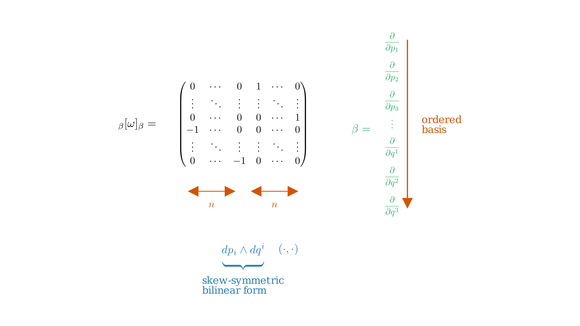
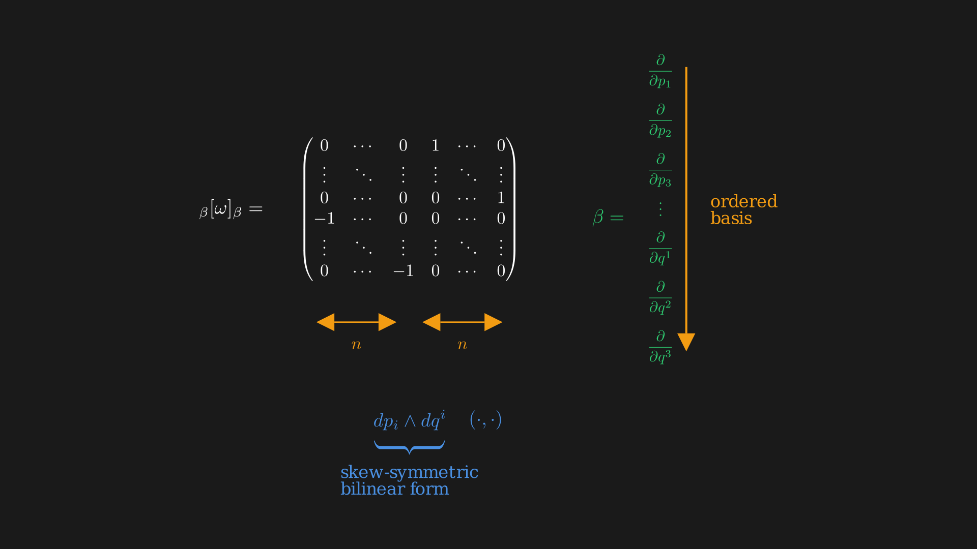
If we plug in the basis vectors $\frac{\partial}{\partial q^i}$ and $\frac{\partial}{\partial p_i}$ in Equation \eqref{eq:skew-symmetric-bilinear-form} we get the matrix. It is easy to see most of the entries are $0$ because we might get non-zero only when the momentum we plug in and the position we put in have the same index.

This gives us some properties of $\omega$,

1. $\omega$ is skew-symmetric, i.e. $\omega(u, v) = -\omega(v, u)$.
2. $\omega$ is closed, i.e. $d\omega = 0$ (notice that $\omega$ is $d(1$-form$)$).
3. $\omega$ is non-degenerate, i.e. $\omega(u, v) = 0$ for all $v \in T_{(q, p)}M$ implies $u = 0$.

This means, we can use it to define a map that takes a tangent vector to a covector on the phase space, $\omega: TM \mapsto T^*M$ or $\omega: u \mapsto \underbrace{\iota_u \omega}_{\text{interior product}} = \omega(u, \cdot)$. The $\cdot$ is a covector on the phase space. Since $\omega$ is non-degenerate, this map is an isomorphism.

\[\begin{equation} \begin{split} \omega:& TM \mapsto T^*M \\ \omega:& u \mapsto \underbrace{\iota_u \omega}_{\text{interior product}} = \omega(u, \cdot) \\ \omega:& \frac{\partial}{\partial p_i} \mapsto \iota_{\frac{\partial}{\partial p_i}} (dp_j \wedge dq^j) = \left( \iota_{\frac{\partial}{\partial p_i}} dp_j \right) dq^j + (-1) dp_j \wedge \underbrace{(\iota_{\frac{\partial}{\partial p_i}} dq^j)}_0 = dq^i \\ \omega:& \frac{\partial}{\partial q^i} \mapsto -dp_i. \\ \end{split} \label{eq:omega-map} \end{equation}\]

So the momentum vector gets sent to the derivative of the position vector. And the position vector gets sent to the negative derivative of the momentum vector. We essentially get to convert a tangent vector on phase space to a cotangent vector on phase space.

Hamiltonian Vector Field of $f$. This essentially gives us a way to convert $f \in C^\infty(M, \mathbb{R})$ to a vector field $X_f \in \Psi(M)$, \begin{equation} f \mapsto \underbrace{df}_{\in \Omega^1(M)} \mapsto -\omega^{-1}(df) = \underbrace{X_f}, \end{equation} where $X_f \in \Psi(M)$ is the Hamiltonian vector field associated to $f$.

The Hamiltonian vector field $X_f$ is such that,

1. Hamiltonian vector field of $f$ preserves itself. $X_f (f) = df (X_f) = df(-\omega^{-1}(df)) = -\omega^{-1}(df, df) = 0$ since $\omega$ is skew. However, this is very different from the gradient of $f$, on a Riemannian manifold $\nabla f = g^{-1}(df)$, $(\nabla f) (f) = df (g^{-1}df) = g^{-1}(df, df) = \mid \mid df \mid \mid^2$. Essentially, if the derivative is non-zero the gradient is not going to preserve the function. The Hamiltonian vector field, on the other hand, preserves the level sets of $f$ or $f$ is conserved by the flow of $X_f$. And this is exactly why things like energy and momentum can be conserved, due to this feature of the Hamiltonian vector field.

2. Differentiating the symplectic form in the direction of the vector field.

\[\begin{equation} \begin{split} L_{X_f} \omega &= (d \iota_{X_f} + \iota_{X_f}d)\omega \\ &= d \iota_{X_f} \omega \\ &= d(\omega (-\omega^{-1}df, \cdot)) \\ &= d (-df) \\ &= 0, \end{split} \end{equation}\]

Thus, $\omega$ is preserved, where $\mathcal{L}$ is the Lie derivative. The Hamiltonian vector field of a function $f$ is a symmetry of $(M, \omega , f)$. So, a Hamiltonian system consists of:

• a manifold $M$ (cotangent bundle of another manifold $X$)
• $\omega$, a symplectic form on $M$ (a non-degenerate, closed $2$-form) ⁵
• a function $H$ or $f$, the Hamiltonian

The Poisson bracket associated to $\omega$ is,

\begin{equation} \lbrace , \rbrace : C^\infty(M, \mathbb{R}) \times C^\infty(M, \mathbb{R}) \mapsto C^\infty(M, \mathbb{R}), \label{eq:poisson-bracket} \end{equation}

so we can take two functions $f$ and $g$ and one of these two functions determines a Hamiltonian vector field and we can use this vector field to differentiate the other function,

\begin{equation} \lbrace f, g\rbrace = \color{red}{X_g(f)} = df (-\omega^{-1}(dg)) = \omega^{-1}(df, dg) = -\omega^{-1}(dg, df) = \color{red}{-X_f(g)}. \end{equation}

The Poisson bracket, Equation \eqref{eq:poisson-bracket} satisfies the Leibniz rule,

\[\begin{equation} \begin{split} \underbrace{\lbrace f_1f_2, g\rbrace }_{\text{differentiate product with vector field from $g$}} &= X_g(f_1f_2) \\ &= X_g(f_1)f_2 + f_1X_g(f_2) \\ &= \lbrace f_1, g\rbrace f_2 + f_1\lbrace f_2, g\rbrace \end{split} \end{equation}\]

(Poisson Algebra.) A Poisson algebra is a commutative algebra $A$ together with a bracket $\lbrace ,\rbrace : A \times A \mapsto A$ that is,

1. skew
2. satisfies the Leibniz rule $\lbrace f, gh\rbrace = \lbrace f, g\rbrace h + g\lbrace f, h\rbrace $
3. satisfies the Jacobi identity $\lbrace \lbrace f, g\rbrace , h\rbrace = \lbrace f, \lbrace g, h\rbrace \rbrace + \lbrace g, \lbrace f, h\rbrace \rbrace $.

Proof that the Poisson bracket satisfies condition 3. Let $f, g, h \in C^\infty(M, \mathbb{R})$. Consider the $1$-parameter family of canonical transformations $\Phi_t$ generated by $h$, i.e. the flow of the Hamiltonian vector field $X_h$. For any observable $F$ set $F_t := F \circ \Phi_t$ and define the infinitesimal variation $\delta F := \left.\frac{d}{dt}\right\rvert_{t=0} F_t$. By our definition of the Poisson bracket and the fact that $X_h$ preserves $\omega$ (we already showed $\mathcal{L}_{X_h}\omega = 0$), we have \begin{equation} \delta F = X_h(F) = \lbrace F, h\rbrace. \label{eq:infinitesimal-variation} \end{equation} On the one hand, because $\Phi_t$ is a symplectomorphism it preserves the Poisson bracket, so \begin{equation} \delta\, \lbrace f, g\rbrace = X_h(\lbrace f, g\rbrace) = \lbrace \lbrace f, g\rbrace, h\rbrace. \label{eq:jacobi-hand-1} \end{equation} On the other hand, the change in $\lbrace f, g\rbrace$ comes only from the changes in $f$ and $g$ themselves. Using bilinearity and $\delta f = X_h(f) = \lbrace f, h\rbrace$ and $\delta g = X_h(g) = \lbrace g, h\rbrace$, we get \begin{equation} \begin{split} \delta\, \lbrace f, g\rbrace &= \lbrace \delta f, g\rbrace + \lbrace f, \delta g\rbrace \\\\ &= \lbrace \lbrace f, h\rbrace, g\rbrace + \lbrace f, \lbrace g, h\rbrace \rbrace. \end{split} \label{eq:jacobi-hand-2} \end{equation} Comparing \eqref{eq:jacobi-hand-1} and \eqref{eq:jacobi-hand-2} yields \begin{equation} \lbrace \lbrace f, g\rbrace, h\rbrace = \lbrace \lbrace f, h\rbrace, g\rbrace + \lbrace f, \lbrace g, h\rbrace \rbrace, \end{equation} which is equivalently the cyclic form \begin{equation} \lbrace \lbrace f, g\rbrace, h\rbrace + \lbrace \lbrace h, f\rbrace, g\rbrace + \lbrace \lbrace g, h\rbrace, f\rbrace = 0, \label{eq:jacobi-identity} \end{equation} exactly the Jacobi identity (condition 3).

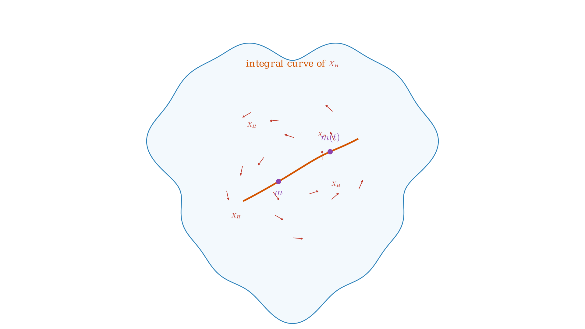
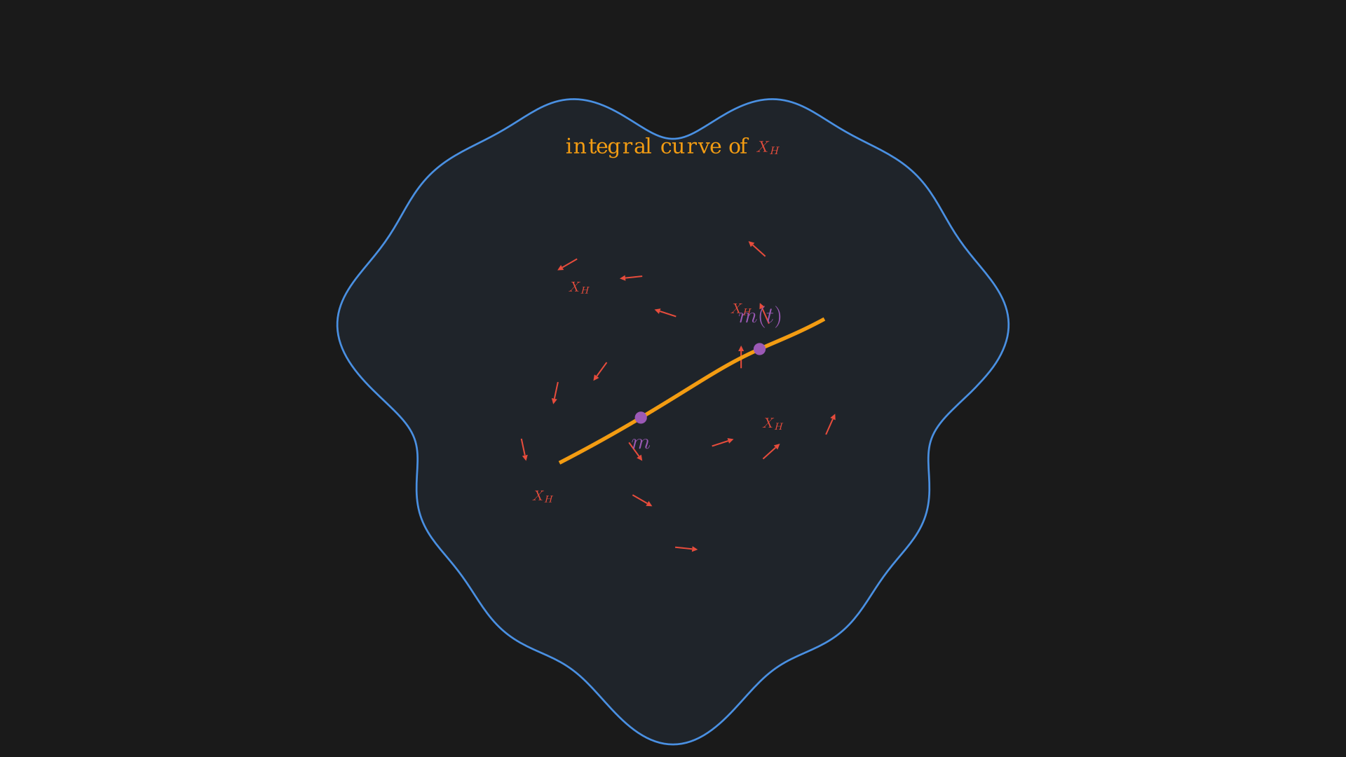
The Poisson bracket is helpful for defining the Hamiltonian flow, we know $C^\infty(M, \mathbb{R}) \ni H \mapsto X_H$ generates a flow, $\Phi_t^{X_H}: (\mathbb{R}, t) \times M \mapsto M$ such that $(t, m) \mapsto \Phi_t^{X_H}(m) = m(t)$ where $\frac{d}{dt}m(t) = X_H(m(t))$.

The Hamiltonian flow as a diffeomorphism on the phase space.

Alternatively, we can flow a function too, $f \in C^\infty(M, \mathbb{R})$ i.e. $f(t) = (\psi_t^{X_H})^*f$ since the flow is anyway a diffeomorphism. What we essentially want is to produce a path of functions such that at every moment in time the change in the function is given by the derivative along the vector field $\frac{d}{dt}f(t) = X_H(f(t)) = \underbrace{\lbrace f, H\rbrace}_{\text{Poisson bracket}}$ (Hamilton’s Equation). Essentially, the equation of motion for a function $f$ dragged along Hamiltonian flow is the Poisson bracket.

In any Poisson algebra $(A, \lbrace ,\rbrace)$ we can write a similar equation. Fix $H \in \mathcal{A}$ then we can write a differential equation for a path $f(t)$ of elements in A: $\dot{f} = \lbrace f, H\rbrace$. We can think of the Hamiltonian flow as acting on every state, so if we choose a state we can see how it evolves in time or also describe a function and see how it evolves in time.

What this means is:

1. If we know the initial state exactly, we can find the evolution $\dot{m}(t) = X_H(m(t))$
2. But if we only have probabilistic information about the state, say a density $\rho$, we can still get $\dot{\rho} = \lbrace \rho, H\rbrace$

Organizing Hamiltonians

Functions on $M=T^*Q$ with some coordinates $(q^i, p_j)$. It does not make sense to classify functions based on the degree of $q$ because that is dependent on the choice of coordinate system we have. But we can organize Hamiltonians based on degree in vector space directions $p_i$.

Degree 0

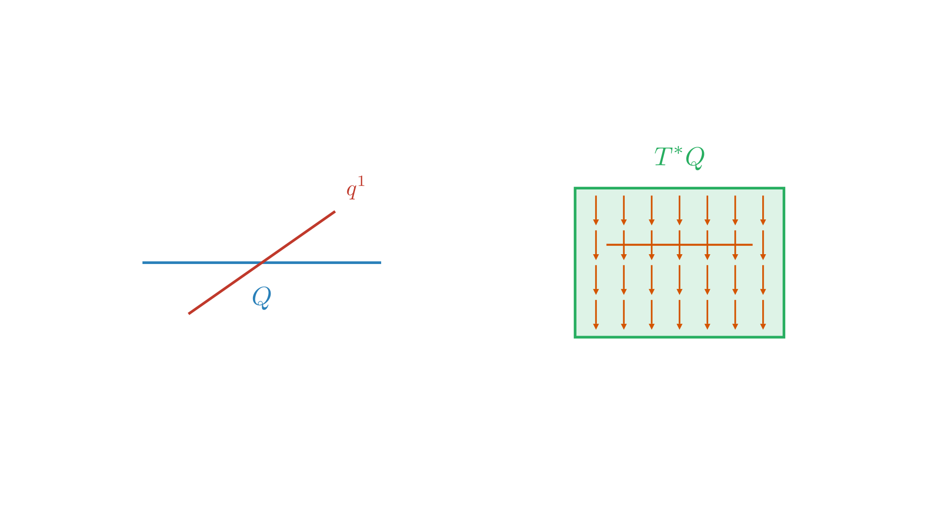
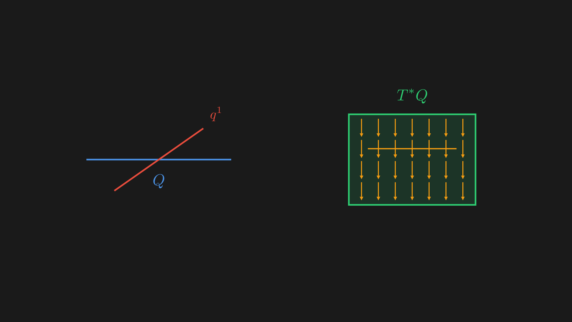
First, we have functions which are constant in cotangent directions so the function is of $q$, not of $p$, $f=V(q^1, \ldots, q^n)$. This is like saying $f$ is pulled back from $V \in C^{\infty}(Q, \mathbb{R})$. So, $M=T^*Q \rightarrow ^{(\pi)} Q \rightarrow ^{(V)} \mathbb{R}$ or $\pi^*V = V \circ \pi: M \to \mathbb{R}$.

If we take $V=q^1$, then $X_v = -\omega^{-1}dV = -\omega^{-1}dq^1 = -\frac{\partial}{\partial p_1}$ (from Equation \eqref{eq:omega-map}). As we expect, the level sets of Hamiltonians are preserved by the Hamiltonian flow. The effect this has is we stay at the same position but our momentum is increased.

The Hamiltonian flow of a degree 0 Hamiltonian.

Degree 1

$f = V^1 p_1 + V^2 p_2 + \cdots + V^n p_n$, this is a linear combination of $p$, the coefficient $V^i$ is any smooth function of $q$, $V^i = V^i(q^1, \ldots, q^n)$. So now, the Hamiltonian vector field of this function is,

\[\begin{equation} \begin{split} X_f &= -\omega^{-1}(df) \\ &= -\omega^{-1}(p_i dV^i + V^i dp_i) \\ &= -\omega^{-1}(p_i \frac{\partial V^i}{\partial q^j} + V^i dp_i) \\ &= -p_i \frac{\partial V^i}{\partial q^j}\frac{\partial}{\partial p_j} + V^i \frac{\partial}{\partial q^i} \\ \end{split} \label{eq:hamiltonian-vector-field-degree-1} \end{equation}\]

We now have a term that has a vertical component $\frac{\partial}{\partial p_j}$ for the Hamiltonian flow depending on the magnitude of the momentum. This guarantees that the Hamiltonian flow has, $\frac{d}{dt}q^i = V^i(q^1, \ldots, q^n)$ because there is only one term changing $q^i$, $V^i \frac{\partial}{\partial q^i}$. We can use the ODE $\frac{d}{dt}q^i = V^i(q^1, \ldots, q^n)$ to directly get the positions in this case.

We can also see how the $p_j$ is changing, $\frac{d}{dt}p_j = -p_i\frac{\partial V^i}{\partial x^j}$. The phase portrait would look like something where the $x$-axis is given by the ODE for $q^i$ and the $y$-axis is given by the ODE for $p_j$.

For example, consider $f=p_1$ which is set $V^1=1$, $V^2=V^3=\cdots=0$. Then, $X_f = -\omega^{-1}(dp_1) = \frac{\partial}{\partial q^1}$ or we don’t have the first term at all in Equation \eqref{eq:hamiltonian-vector-field-degree-1}. This is another way of saying the momentum function generates spatial translation or when we flow along the Hamiltonian vector field for time $t$,

\[\begin{equation} \Psi_t^{X_f}: (q, p) \mapsto (q + \underbrace{(t, 0, \ldots, 0)}_{\text{translate in $q^1$ direction}}, p) \end{equation}\]

We can think of this as for degree $0$ we have functions on $Q$, $C^\infty(Q)$ and for degree $1$ we have vector fields on $Q$, $\mathfrak{X}(Q) = \underbrace{\Gamma(Q, TQ)}_{\text{section of tangent bundle of }Q}$.

The Hamiltonian flow of a degree 1 Hamiltonian.

The function we have is linear in the direction of the fiber so it is $0$ in the zero section of the cotangent bundle and grows linearly in the direction of the fiber. Because of this, they are elements of the dual space of the cotangent fiber and thus are tangent vectors. Since $f\in C^\infty(T^*Q)$ is linear on $T^*Q$ fibers, it defines a tangent vector at every point in $Q$. Thus, Hamiltonians of degree 1 are $\mathfrak{X}(Q)$, vector fields on $Q$. Like, $f = V^1 p_1 + \ldots + V^n p_n$ corresponds to the vector field $V = V^i \frac{\partial}{\partial q^i}$.

(Proposition.) There is a vector field $V$ on $Q$ which generates a flow on $Q$, it induces a diffeomorphism on $Q$. This means it also induces a diffeomorphism on $T^\*Q$. This induced diffeomorphism or symmetry is the Hamiltonian flow of the function determined by $V$.

Hamiltonian flow of $f_V = V^ip_i$ coincides with the flow on $T^\*Q$ induced by the flow of $V$ on $Q$.

Degree 2

Here, we have $f = V^{ij}p_ip_j$, $V^{ij} \in C^\infty(Q)$. To specify this function we need to specify the coefficients $V^{ij}$ so we need $\frac{1}{2}n(n+1)$ smooth functions of $q^1, \ldots, q^n$.

For example, let us suppose we are given a Riemannian metric $g$ on $Q$. We have a tensor $g = g_{ij}(q^1, \ldots, q^n)dq^i \otimes dq^j$ where the $g_{ij}$ term is a symmetric matrix of $n \times n$ smooth functions of $q^1, \ldots, q^n$, is non-degenerate at every point, and positive definite. Without talking about coordinates we can say $g$ defines a map $g: TQ \mapsto T^*Q$ which is an isomorphism. Any vector $v$ we put in $g$ gives us some covector $g(v, \cdot)$. We also have $g^{-1}: T^*Q \mapsto TQ$ which takes in two inner forms to compute an inner product of, $g^{-1} = g^{ij} \frac{\partial}{\partial q^i} \otimes \frac{\partial}{\partial q^j}$ where $g^{ij}$ is the inverse of $g_{ij}$. This defines a quadratic function $\frac{1}{2}f_{g^{-1}} = \frac{1}{2}g^{ij}(q^1, \ldots, q^n)p_ip_j$.

What this means is if you take $Q$ and have the tangent spaces at each point $T^*Q$. On $Q$ where $p=0$ the function is $0$ and on $T^*Q$ where $p \neq 0$ the function grows quadratically as we move on $T^*Q$ so we get ellipsoids or level sets of $fg^{-1}$. Connecting many of these level sets across different points of $Q$ we get cylindrical level sets of $fg^{-1}$ are called the cosphere bundles inside $T^*Q$.

The cosphere bundle.

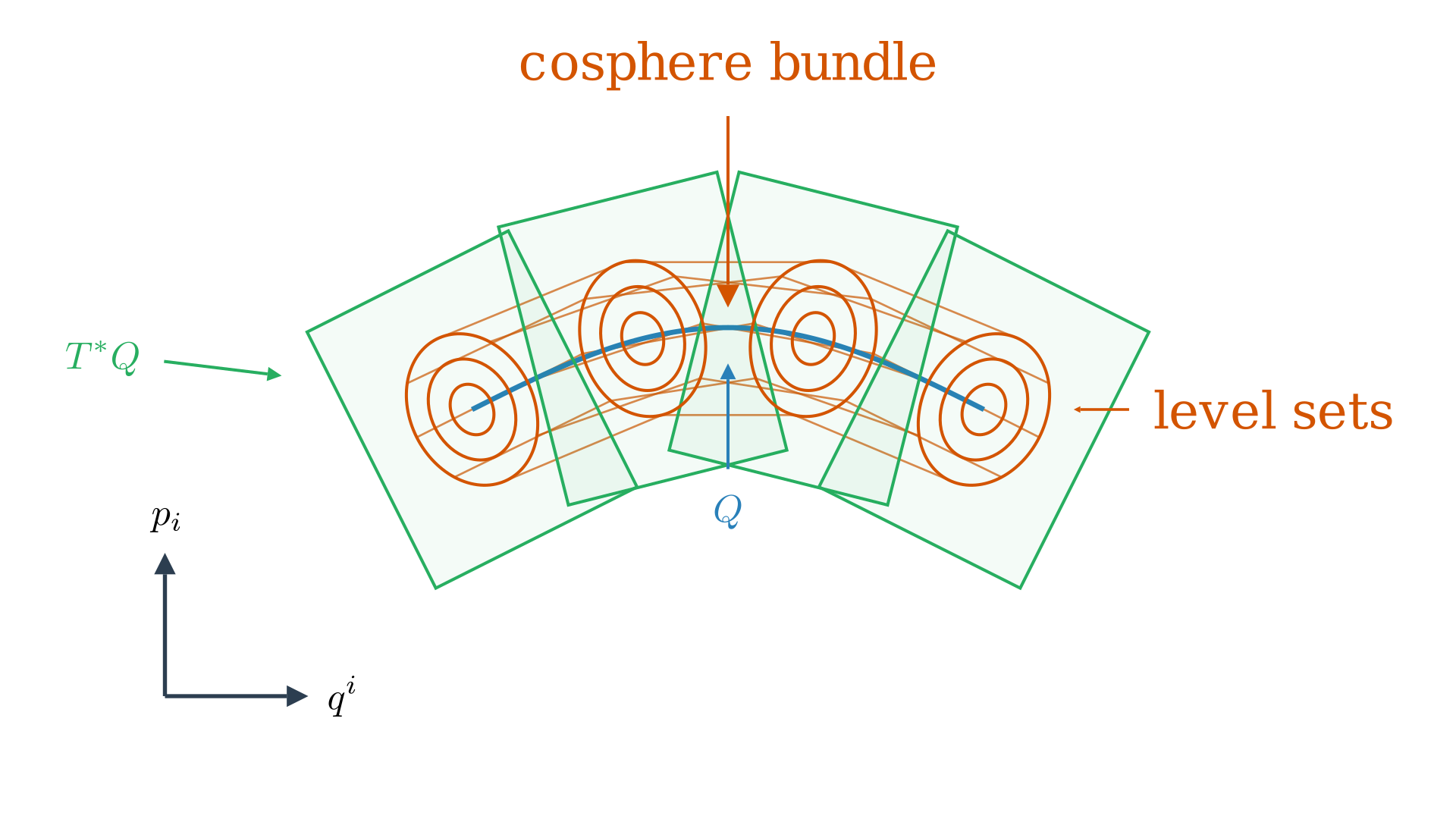
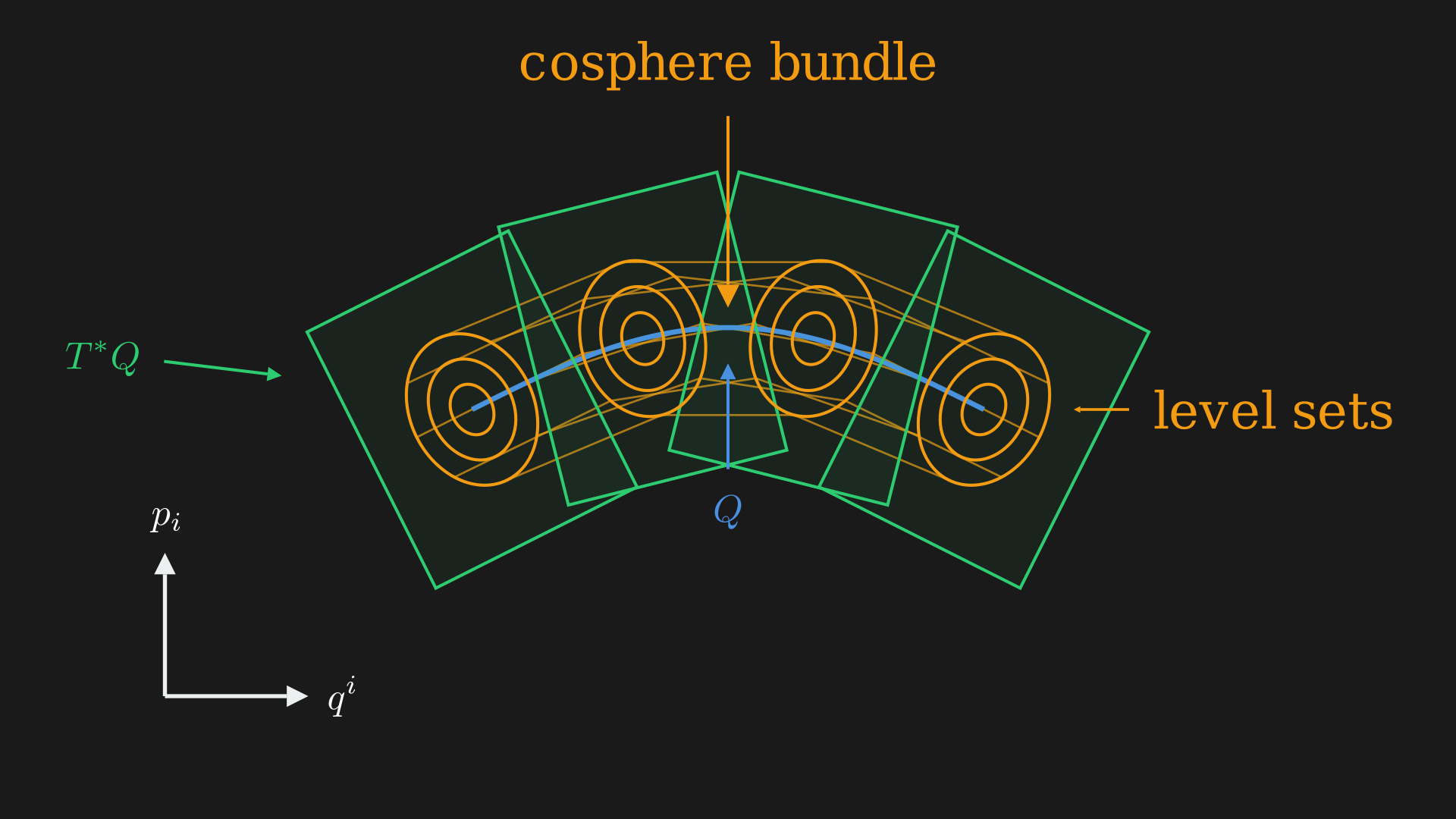
Now, we can think about the Hamiltonian flow of $f_{g^{-1}}$ defined by the Riemannian metric $g$. If you are inside the cosphere bundle on the phase space and as the Hamiltonian flow progresses we will stay inside the cosphere bundle, and the Riemannian metric or the norm-squared of the momentum is preserved. Interestingly, this function $\frac{1}{2}f_{g^{-1}}$ is the exact definition of kinetic energy of a particle on $Q$ (this definition works on any Riemannian manifold).

The Hamiltonian is,

\[\begin{equation} \begin{split} H &= \frac{1}{2}g^{ij}(q^1, \ldots, q^n)p_ip_j\\ dH&= \frac{1}{2} d(g^{ij}(q^1, \ldots, q^n)p_ip_j) p_i dp_j + \frac{1}{2} g^{ij}(q^1, \ldots, q^n)p_i dp_j\\ &= \frac{1}{2} \frac{\partial g^{ij}}{\partial q^k}p_ip_j dq^k + \frac{1}{2} g^{ij}(q^1, \ldots, q^n)p_i dp_j\\ -\omega^{-1}(dH)&= \frac{1}{2} \frac{\partial g^{ij}}{\partial q^k}p_ip_j dq^k\frac{\partial}{\partial p_k} + \frac{1}{2} g^{ij}(q^1, \ldots, q^n)p_i \frac{\partial}{\partial q^j} \end{split} \label{eq:hamiltonian-degree-2} \end{equation}\]

So, we have the ODEs

\[\begin{equation} \begin{split} \dot{q}^j &= g^{ij}p_i \\ \dot{p}_j &= -\frac{1}{2}\partial_k g^{ij}p_i p_j \end{split} \label{eq:hamiltonian-degree-2-ode} \end{equation}\]

One very interesting way of thinking about this is, compare the definition of kinetic energy to $\frac{1}{2}mv^2$ then the Riemannian metric $g$ is the analog of the mass. What the Hamiltonian flow is growing with $p$ in the horizontal direction, which is like saying if our momentum is large we need to move faster at the same mass.

It turns out that to get a physically meaningful interpretation, we actually need to start with this degree $2$ Hamiltonian which makes the relation between the momentum and the velocity clear.

However, there is one thing we need to be careful of. Let us see Equation \eqref{eq:hamiltonian-degree-2}, it says for momentum ODE the derivative of it is related to square of the momentum. This is like the non-linear ODE Riccati equation $\dot{y} = y^2$. The Riccati equation goes to $\infty$ in a finite time. And this problem can exist in the vector field as well, the velocity can go to $\infty$ in finite time under the flow. This eerily reminds me of Lagrangian mechanics where we use time integrators like Forward Euler which have exactly the same problem.

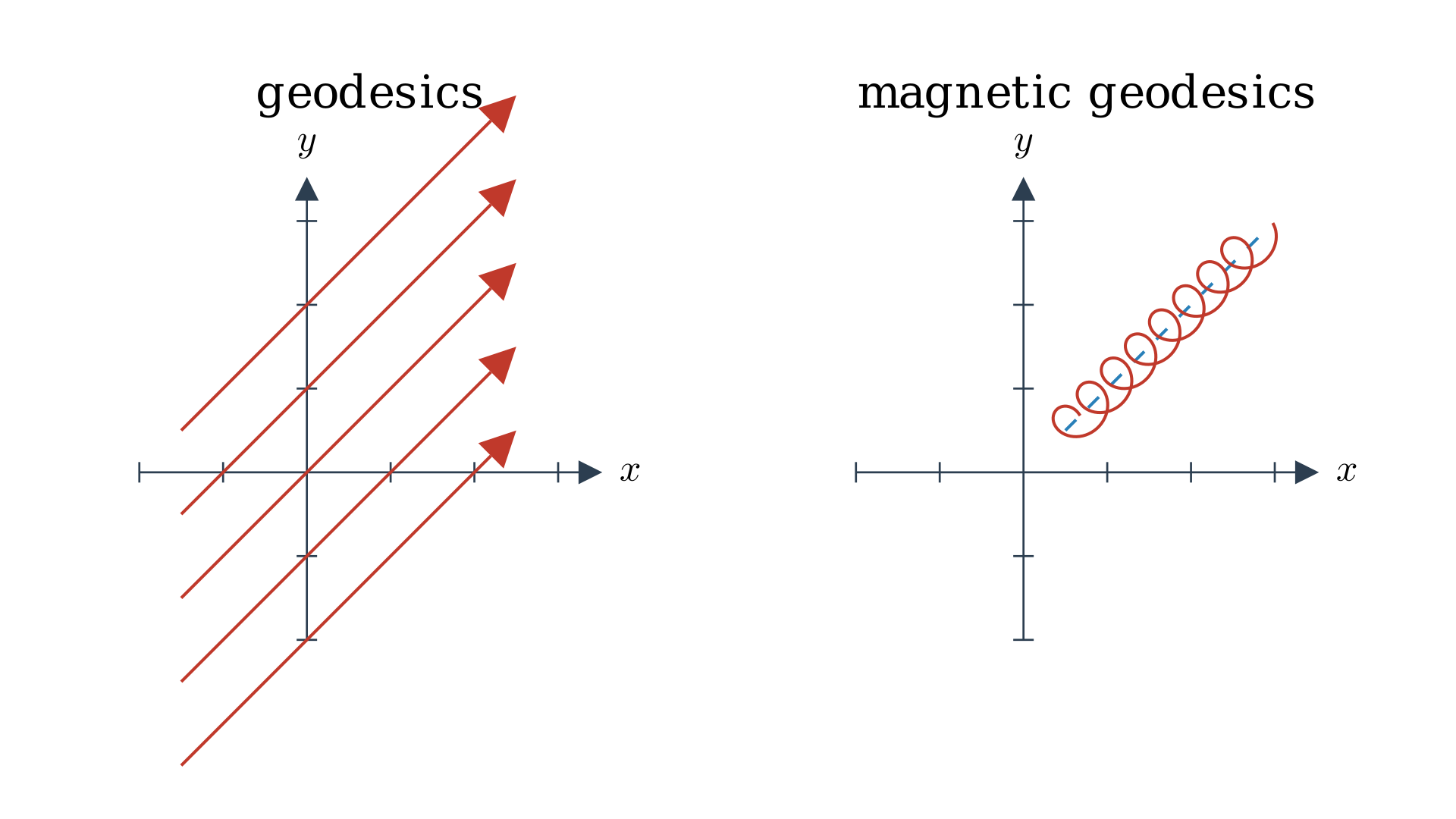
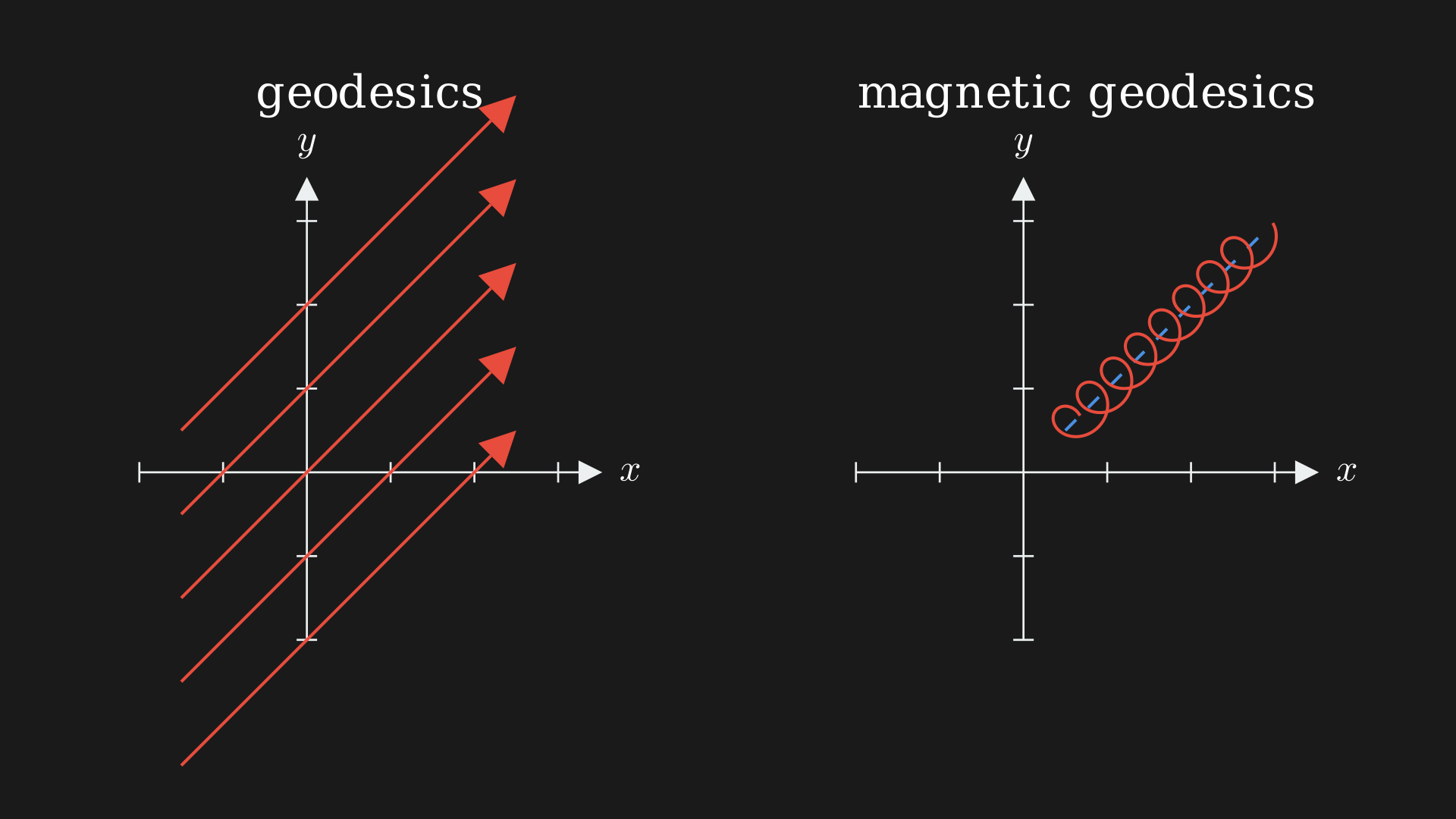
If the flow exists for all time, we say $(Q, g)$ is a complete Riemannian manifold. The solutions $(q(t), p(t))$ determine parameterized curves $q(t)$ in $Q$. These curves are geodesics on the original Riemannian manifold. The geodesic equation is actually Hamiltonian! We can write the geodesic equation as,

\[\begin{equation} \gamma: \mathbb{R} \mapsto (Q, g) \end{equation}\]

where $\gamma$ is the parametric curve in $Q$. $\dot{\gamma} \in \Gamma(\mathbb{R}, \gamma^*TQ)$. The standard Levi-Civita connection is $\nabla_{\frac{\partial}{\partial t}} \dot{\gamma} = 0$ or acceleration is zero; that is, $\gamma(t) = (q^1(t), q^2(t), \ldots, q^n(t))$. The geodesic equation says,

\[\begin{equation} \ddot{q}^i + \Gamma^i_{jk} \dot{q}^j \dot{q}^k = 0 \label{eq:geodesic-equation} \end{equation}\]

where $\Gamma^i_{jk}$ is the Christoffel symbol $\Gamma^i_{jk} = \frac{1}{2} g^{im}(\frac{\partial g_{mj}}{\partial q^k} + \frac{\partial g_{mk}}{\partial q^j} - \frac{\partial g_{jk}}{\partial q^m})$. As it turns out, after some work, the geodesic equation is exactly equivalent to the second degree ODEs in Equation \eqref{eq:hamiltonian-degree-2-ode}.

We can think of this as follows: to analyze geodesic equations, all we can do is have the metric determine a function on the cotangent bundle and that function determines a flow. This flow is the geodesic flow.

What do we get from these degrees?

• Degree 0: Function on the configuration space $V \in C^\infty(X, \mathbb{R})$ (potential)
• Degree 1: Vector fields on the configuration space, $Y \in \mathfrak{X}$
• Degree 2: $T_g = \frac{1}{2} f_g^{-1}$ with a Riemannian metric $g$ (kinetic energy)

An example is taking the degree $0$ and the degree $2$ and putting them together,

\[\begin{equation} \begin{split} H &= T_g + V \\ \underbrace{X_H}_{\text{Hamiltonian vector field}} &= \overbrace{X_g}^{\text{geodesic vector field}} + \underbrace{X_v}_{\text{deflection due to forces from the potential field}} \end{split} \label{eq:hamiltonian-degree-0-and-2} \end{equation}\]

From Hamilton's equations of motion we know, $$ \begin{equation} \begin{split} \dot{q}^i &= \{q^i, H\} \\ \dot{p}_i &= \{p_i, H\} \end{split} \label{eq:hamiltonian-degree-0-and-2-ode} \end{equation} $$

For $X_g$ we have,

\[\begin{equation} \begin{split} X_g:&\qquad \dot{q} = g^{-1}p \\ &\qquad \dot{p}_i = \frac{1}{2}\partial_k g^{ij}p_i p_j \end{split} \end{equation}\]

For $X_v = -\omega^{-1}(dV) = (dp_i \wedge dq^i)^{-1}(\partial_k V dq^k)$ we have,

\[\begin{equation} \begin{split} X_v:&\qquad \dot{q} = 0 \\ &\qquad \dot{p} = -\frac{\partial V}{\partial q^i} \end{split} \end{equation}\]

Using the Levi-Civita connection we get,

\[\begin{equation} \begin{split} &\nabla_{\frac{\partial}{\partial t}} \dot{q} = -\overbrace{g^{-1} (dV)}^{\operatorname{grad}(V)} = g^{-1}F \\ \implies & F = ga = g \nabla_{\frac{\partial}{\partial t}} \dot{q} \end{split} \end{equation}\]

This system takes a force using the potential $V$ and the Riemannian metric $g$ is the equivalent of the mass. If you look at this example, it recovers all Newtonian systems.

An Oscillator

Let us consider a simple oscillator. At this stage, I highly recommend reading my article on the simulation first where I talk about many of these kinds of systems at length.

An example of a simple configuration.

Equip $X$ with Riemannian metric $g$ where $g = m dq \otimes dq$. Here the metric tensor is just the $1 \times 1$ identity matrix, so $T_g=\frac{1}{2}mp^2$. We also need to provide a law of force for a spring, from Hooke’s law we have $V=\frac{1}{2}kq^2$.

The Hamiltonian for this system, or for $X= (\mathbb{R}, q)$ and $T^*X= (\mathbb{R} \times \mathbb{R}, (q,p))$ is,

\[\begin{equation} H = \frac{1}{2}m^{-1}p^2 + \frac{1}{2}kq^2 \end{equation}\]

The Hamiltonian vector field is,

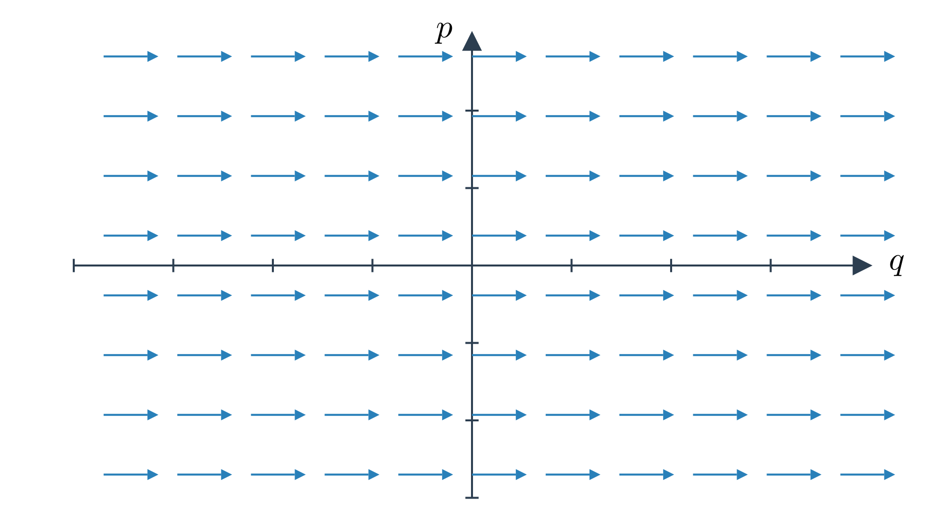
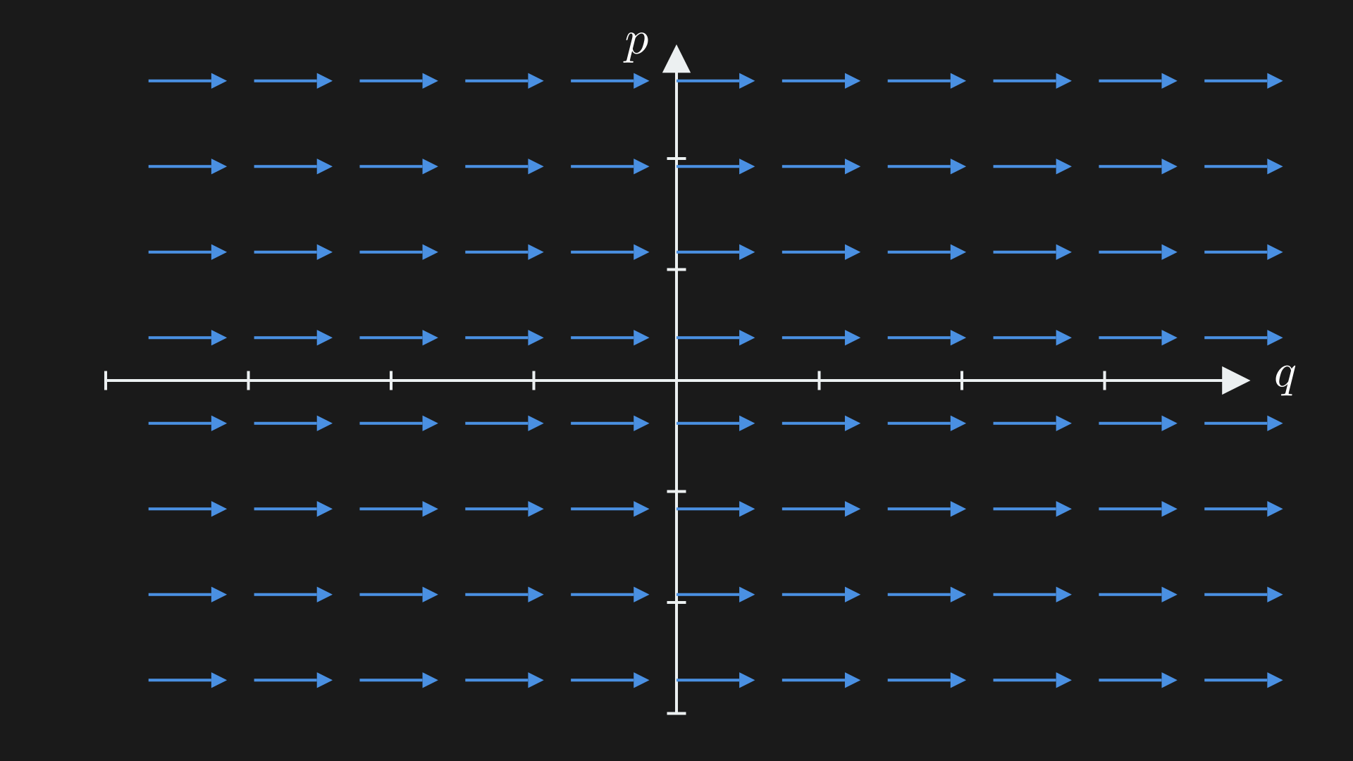
\[\begin{equation} X_H = m^{-1}p \frac{\partial}{\partial q} - kq \frac{\partial}{\partial p} \label{eq:hamiltonian-vector-field-oscillator} \end{equation}\]

The vector field would be a rotational vector field, something like the below image taken from my article on the simulation (you should read this to directly connect this view to the Lagrangian view). Essentially, the vector field gets bigger as we move away from the origin.

The vector field for the oscillator.

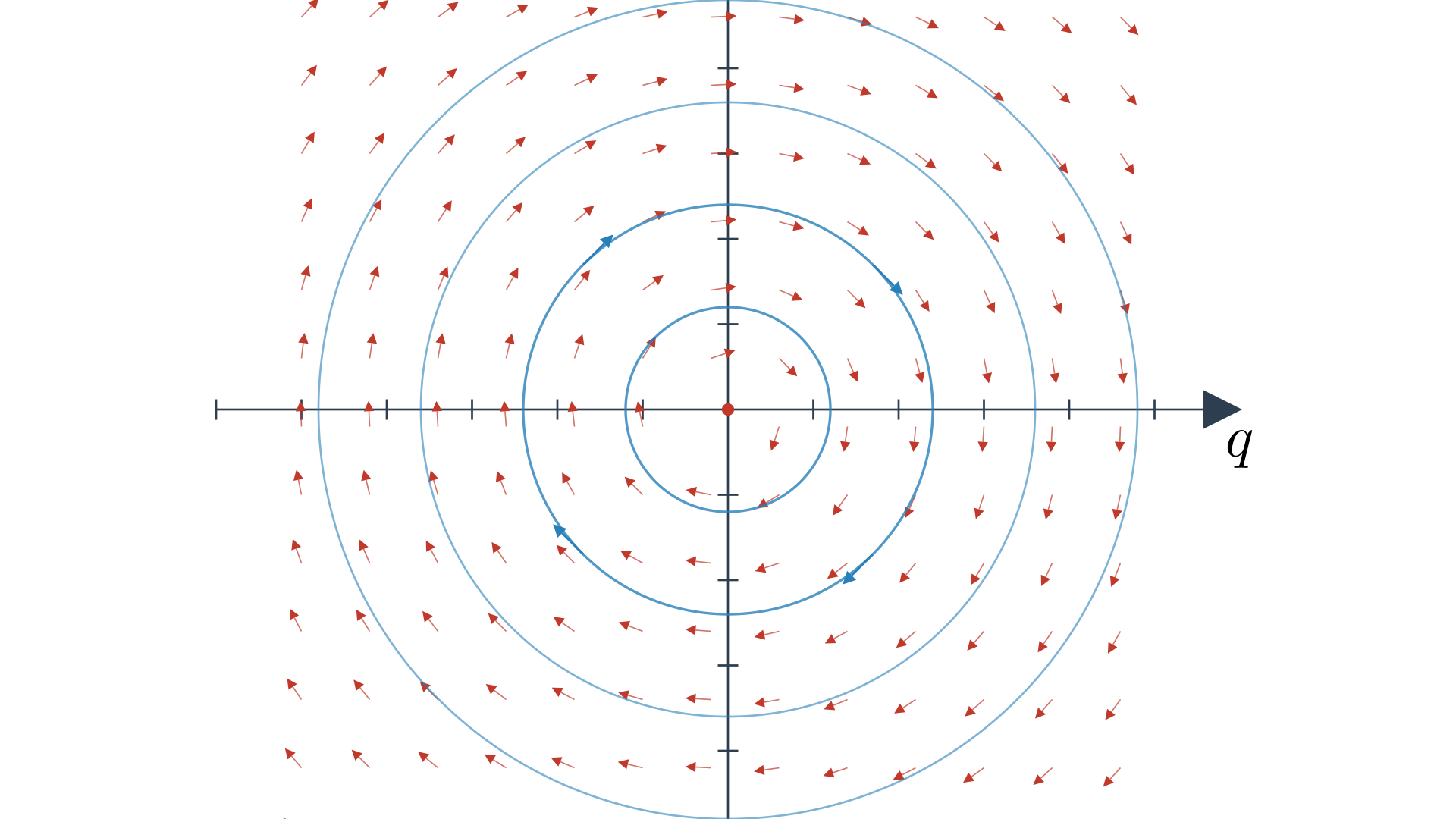
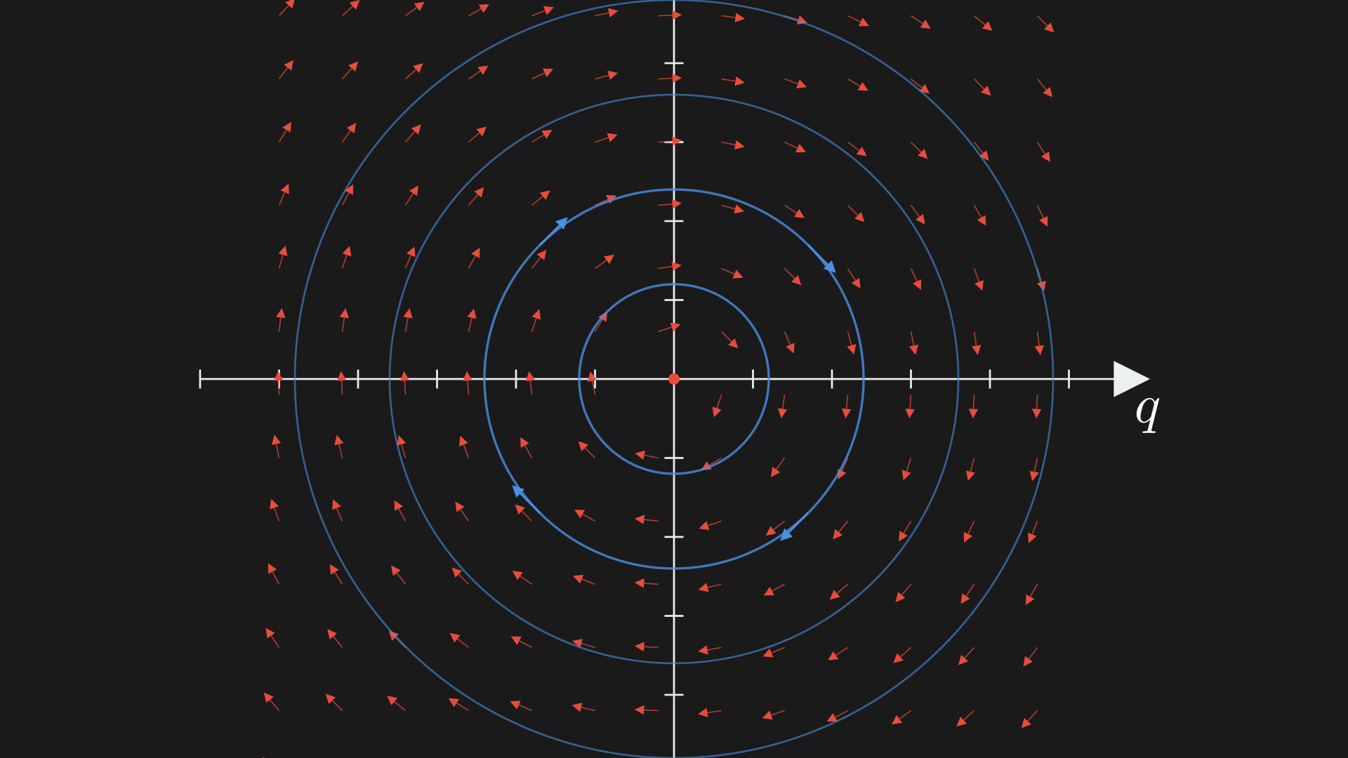
An interesting thing to note here is that the vector field (Equation \eqref{eq:hamiltonian-vector-field-oscillator}) is linear which makes it scale linearly as we scale the points in the cotangent bundle. In this case, the cotangent bundle is a vector space. So, we can represent Hamilton’s equations in matrix form as,

\[\begin{equation} \frac{d}{dt} \begin{pmatrix} q \\ p \end{pmatrix} = \underbrace{\begin{pmatrix} 0 & m^{-1} \\ -k & 0 \end{pmatrix}}_{A} \begin{pmatrix} q \\ p \end{pmatrix} \end{equation}\]

The solution to this is,

\[\begin{equation} \begin{pmatrix} q(t) \\ p(t) \end{pmatrix} = e^{At} \begin{pmatrix} q(0) \\ p(0) \end{pmatrix} \label{eq:solution-oscillator} \end{equation}\]

Does this look familiar? It is exactly what we get from the Lagrangian view! Similarly, note that $A^2 = -k m^{-1} \mathbb{I} = -\omega^2 \mathbb{I}$ so we can scale $A$ such that it squares to the negative of the identity matrix or the operator behaves like a complex number $(\underbrace{\omega^{-1} A}_J)^2=-\mathbb{I}$. So,

\[\begin{equation} (\omega^{-1} A) = J = \left(\sqrt{\frac{k}{m}}\right)^{-1} \begin{pmatrix} 0 & m^{-1} \\ -k & 0 \end{pmatrix} = \begin{pmatrix} 0 & \frac{1}{\sqrt{km}} \\ -\sqrt{km} & 0 \end{pmatrix} \end{equation}\]

So looking at the solution (Equation \eqref{eq:solution-oscillator}) we can write it using Euler’s formula ($e^{i\theta} = \cos(\theta) + i\sin(\theta)$),

\[\begin{equation} \begin{pmatrix} q(t) \\ p(t) \end{pmatrix} = e^{twJ} \begin{pmatrix} q(0) \\ p(0) \end{pmatrix} = \left(\cos(\omega t) \mathbb{I} + \sin(\omega t) J\right) \begin{pmatrix} q(0) \\ p(0) \end{pmatrix} \end{equation}\]

So, $q(t) = \cos(\omega t) q(0) + \underbrace{\frac{1}{\sqrt{km}} \sin(\omega t) p(0)}_{\omega^{-1}\sin{\omega t}\dot{x}(0)}$. An example is if you pull a mass and leave it, we won’t have the second term because the initial velocity is $0$, and we will oscillate with the cosine term at frequency $\omega$.

The Hamiltonian is a function on the phase space, $H \in C^\infty(T^*X) \supset \bigoplus_{k \geq 0} \Gamma(X, \underbrace{\operatorname{Sym}^k(T^*X)}_{\text{polynomial functions } p \text{ of degree }k})$.

Here we can simply change variables or perform a symplectomorphism to eliminate some variables, use $\tilde{q} = \sqrt{k}q$ and $\tilde{p} = \frac{1}{\sqrt{k}} p$, so $H = \frac{1}{2}m^{-1}(k\tilde{p})^2 + \frac{1}{2}\tilde{q}^2$.

This system has a few pretty well-known properties in $k=m=1$,

• all of its trajectories are closed curves in the phase space
• the periods are all given by $T=\frac{2\pi}{\omega}$

We get the period by integrating over one cycle $\int dt = T$ by fixing the energy $H^{-1}(E)$. If we use coordinate $x$ on curve $e$ then $T=\int_e \frac{dx}{{x,H}}$ and remember ${\cdot}$ is the Poisson bracket. We have, ${x,p} = \frac{\partial x}{\partial x}\frac{\partial p}{\partial p} - \frac{\partial x}{\partial p}\frac{\partial p}{\partial x} = 1$ and ${x,x} = 0$. Also, ${x, \frac{1}{2}(p^2+x^2)} = 2 \frac{1}{2}p {x,p} = p$. Further, given $\frac{1}{2} (x^2+p^2) = E$ we have $T = \int_e \frac{dx}{\sqrt{2E-x^2}}$.

Now split the circle curve into two.

The energy level circle and the two curves.

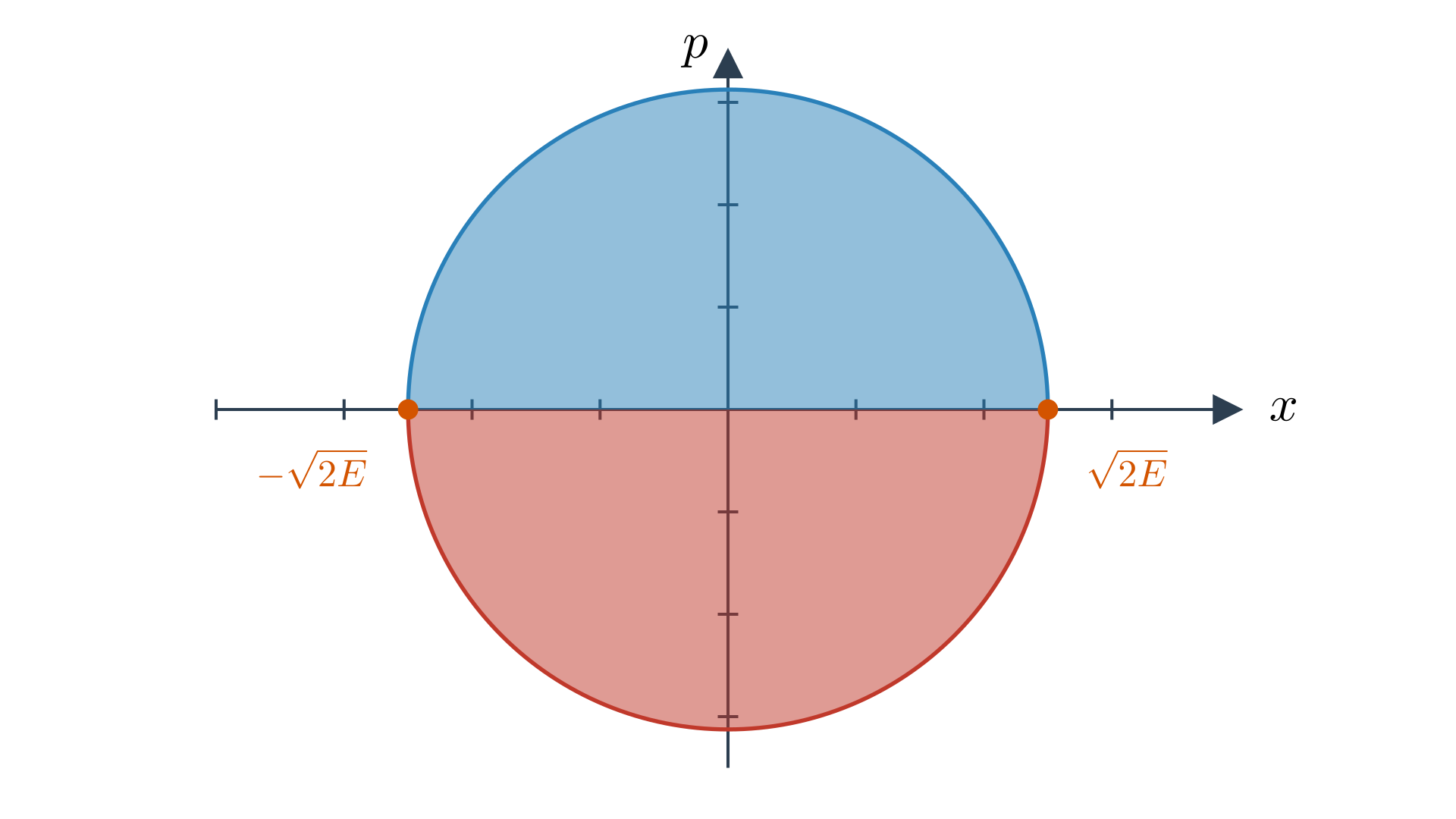
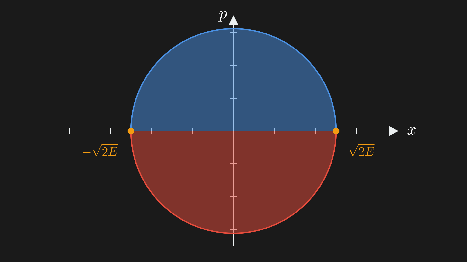
and we end up with $T = 2 \int_{-\sqrt{2E}}^{\sqrt{2E}} \frac{dx}{\sqrt{2E-x^2}} = 2\pi$. This is super interesting because we start out with algebraic data, this algebraic data determines a flow which determines an integral that gives rise to a transcendental number from simple algebraic operations.

Magnetic Deformation

Currently, we can incorporate electric forces from the potential $V (q)$. But a magnetic field is a bit more tricky. A magnetic field $B \in \Omega^2(X)$ is a $2$-form on $X$, $B = B_{ij}(q^1, \ldots, q^n)dq^i \otimes dq^j$ where $B_{ij}$ is a skew-symmetric matrix of $n \times n$ smooth functions of $q^1, \ldots, q^n$. We also need $dB=0$.

To incorporate the magnetic field we need to change the canonical symplectic form $\omega \in \Omega^2(T^*X)$ somehow. We need to somehow deform and change the symplectic form. One thing we can do is shift $\omega$ to $\omega + \pi^*B$ and then $\omega_B= dp_i \wedge dq^i + B_{ij} dq^i \wedge dq^j$. It is hard to see $\omega_B$ is symplectic because it needs to be closed (which is easy to show), skew-symmetric (which is easy to show), and non-degenerate.

The $\omega_B$ defines a bundle map, $\omega_B: TM \mapsto T^*M$, $v \mapsto \iota_v \omega_B = \omega_B(v, \cdot)$. This should be isomorphic. We can check that $det(\omega_B)_{ij} \neq 0$. In the case of skew-symmetric matrix the determinant of the matrix is the square of the Pfaffian $(Pf(\omega_B))^2$.

The Pfaffian is essentially just $\frac{1}{n!} \omega_B \wedge \omega_B \wedge \cdots \wedge \omega_B \in \Omega^{2n}(M) = \underbrace{\frac{1}{n!} \omega_B^n}_{\text{Liouville volume form}}$. This means $\omega_B$ is non-degenerate if $\frac{1}{n!} \omega_B^n$ is nowhere zero.

We can now use the change in variables we made giving us $\omega_B$,

\[\begin{equation} \omega_B^n = (\omega + \pi^*B)^n = \omega^n + n \omega^{n-1} \wedge B + {n \choose 2} \omega^{n-2} \wedge B^2 + \cdots + B^n \label{eq:omega-b} \end{equation}\]

We can call something like $B$ type $(0, 2)$ because it has $2$ q’s, $B=B_{ij}dq^i \wedge dq^j$. Here, when we do $\omega^{n-1} \wedge B$ we have type $(n-1, n-1)$ for $\omega^{n-1}$ and $(0,2)$ for $B$ so $\omega^{n-1} \wedge B$ is type $(n-1, n+1)$. The $\omega^{n-1} \wedge B$ term is a wedge product of $n+1$ $dq^i$’s, so we have $dq^1 \ldots dq^n$ and then one more $dq^k$ term. Remember the exterior product is alternating so the $dq^k$ would be equal to something else and $\omega^{n-1} \wedge B = 0$. Similarly, $\omega^{n-k} \wedge B^k=0$. In Equation \eqref{eq:omega-b} we have, all the terms after $\omega^n$ are $0$.

Thus, $\omega_B$ is symplectic and has the same Liouville volume as $\omega$.

If $(X, g)$ is a Riemannian manifold then the Hamiltonian system defines the free motion of particles by geodesics $(T^*X, \omega, H=\frac{1}{2}f_g^{-1})$.

Similarly if $B \in \Omega^2(X)$ and $dB=0$ then the Hamiltonian system defines the motion of charged particles in a magnetic field $(T^*X, \omega_B = \omega + \pi^*B, H=\frac{1}{2}f_g^{-1})$.

Poisson Bracket

The Hamiltonian flow is $X_H = -\omega_B^{-1}(dH)$ Let us start by computing the inverse to obtain the Poisson bracket:

\[\begin{equation} \begin{split} \omega_B^{-1} &= (\omega + \pi^*B)^{-1} \\ &= (\omega (1 + \omega^{-1}B))^{-1} \\ &= (1+ \omega^{-1}B)^{-1} \omega^{-1} \\ &= (1 - \omega^{-1}B + \omega^{-2}B^2 - \cdots) \omega^{-1} \\ &= \omega^{-1} - \omega^{-1}B \omega^{-1} + \omega^{-1}B\omega^{-1}B\omega^{-1} - \cdots. \end{split} \label{eq:omega-b-inverse} \end{equation}\]

Remember $\omega: T \mapsto T^*$ and $B: T \mapsto T^*$ or $\frac{\partial}{\partial q^i} \mapsto B_{ij} \frac{\partial}{\partial q^j}$.

So if we think of the sequence we have, $B \omega^{-1}B$, then $\frac{\partial}{\partial q^i} \mapsto B_{ij} \frac{\partial}{\partial q^j} \mapsto B_{ij}\frac{\partial}{\partial p_j} \mapsto 0$. So all the terms after $\omega^{-1}B\omega^{-1}$ in Equation \eqref{eq:omega-b-inverse} are $0$.

So, the Hamiltonian vector field changes to $\omega_B^{-1} = \omega^{-1} - \underbrace{\omega^{-1}B \omega^{-1}}_{\text{new magnetic force}}$. This new Hamiltonian vector field does not change the $q$’s but it does change the $p$’s.

\[\begin{equation} \begin{split} \omega_B^{-1} &: dq^i \mapsto \frac{\partial}{\partial p^i} \\ &: dp^i \mapsto -\frac{\partial}{\partial q^i} + B_{ij} \frac{\partial}{\partial p^j} \end{split} \end{equation}\]

So, our solutions change to,

\[\begin{equation} \begin{split} \dot q = g^{-1}p &\rightarrow \dot q = g^{-1}p \\ \dot p = \frac{1}{2}\partial_k g^{ij}p_i p_j &\rightarrow \dot p = \frac{1}{2}\partial_k g^{ij}p_i p_j +p_jg^{ij}B_{ik} \end{split} \end{equation}\]

These new solutions are the magnetic geodesics. Similar to earlier, the acceleration $\nabla_{\dot{q}} \dot{q} = g^{-1} (\iota_{\dot{q}} B)$ is the inverse mass multiplied by the magnetic force. Again, the $g$ acts as the mass.

Particle in $\mathbb{R}^2$

As an example, consider a free particle in the configuration space $(\mathbb{R}^2, x, y) = X$. The cotangent space $T^*X = \mathbb{R}^2 \times \mathbb{R}^2$ with coordinates $(x, y, p_x, p_y)$ with $B = dx \wedge dy$. For the Riemannian metric on $\mathbb{R}^2$ we have $g = dx^2 + dy^2$. So, the Hamiltonian is $H = \frac{1}{2} (p_x^2 + p_y^2)$.

Now, we can consider magnetic deformation $\omega_B = dp_x \wedge dx + dp_y \wedge dy + b dx \wedge dy$.

Comparing solutions to the geodesic equation with and without a magnetic field.

Incorporating Relativistic Effects

This mathematical model is very interesting because it lets us easily incorporate many other physical phenomena, such as magnetic fields and, here, even relativity, into the same framework. Let us see now how we can incorporate relativity into this.

We have $X$ as the configuration space and time as $\mathbb{R}$. We can define a new extended configuration space $(X \times \mathbb{R}, (x, t))$. From this, we can get the extended phase space,

\[\begin{equation} T^*(X \times \mathbb{R}) = \underbrace{T^*X}_{(x, p)} \times \underbrace{T^*\mathbb{R}}_{(s, t)}. \label{eq:extended-phase-space} \end{equation}\]

We can interpret Equation \eqref{eq:extended-phase-space} as $p$ being the momentum in the configuration space (spatial momentum) while $s$ is the momentum in the time direction (timelike momentum).

One of the things to note here is we can’t just have a Riemannian metric on the extended phase space to govern the system; instead, we have a Lorentzian metric on the extended phase space, $g_X - dt^2$ where $g_X$ is the Riemannian metric on the configuration space $X$ and $dt^2$ is the standard metric on $\mathbb{R}$. The signature of the metric is,

\[\begin{equation*} \begin{pmatrix} -1 & 0 \\ 0 & \mathbb{I}_{n \times n} \end{pmatrix} \end{equation*}\]

which is a bilinear form at each event $(x, t)$.

Just like we had earlier the Lorentzian metric determines a quadratic function on the extended phase space,

\[\begin{equation} f_{g_{\text{Lorentzian}}} = \underbrace{\frac{1}{2} g^{ij}(x)p_ip_j}_{\text{kinetic energy along spatial directions}} - \overbrace{\frac{1}{2} s^2}^{\text{kinetic energy along time direction}}. \end{equation}\]

If we use $H = f_{g_{\text{Lorentzian}}}$ to generate flows we obtain the Lorentzian geodesics. The initial condition we have is $((x, t), (p,s))$, the norm \(\|p\|^2 - s^2 = -m^2\) may be positive (space-like), negative (time-like), or zero (light-like). If you have read the popular book, “A Brief History of Time” by Hawking, you might find much of this familiar. You can interpret this flow as follows, again shamelessly copied from “A Brief History of Time”.

The light cone (shamelessly copied from A Brief History of Time).

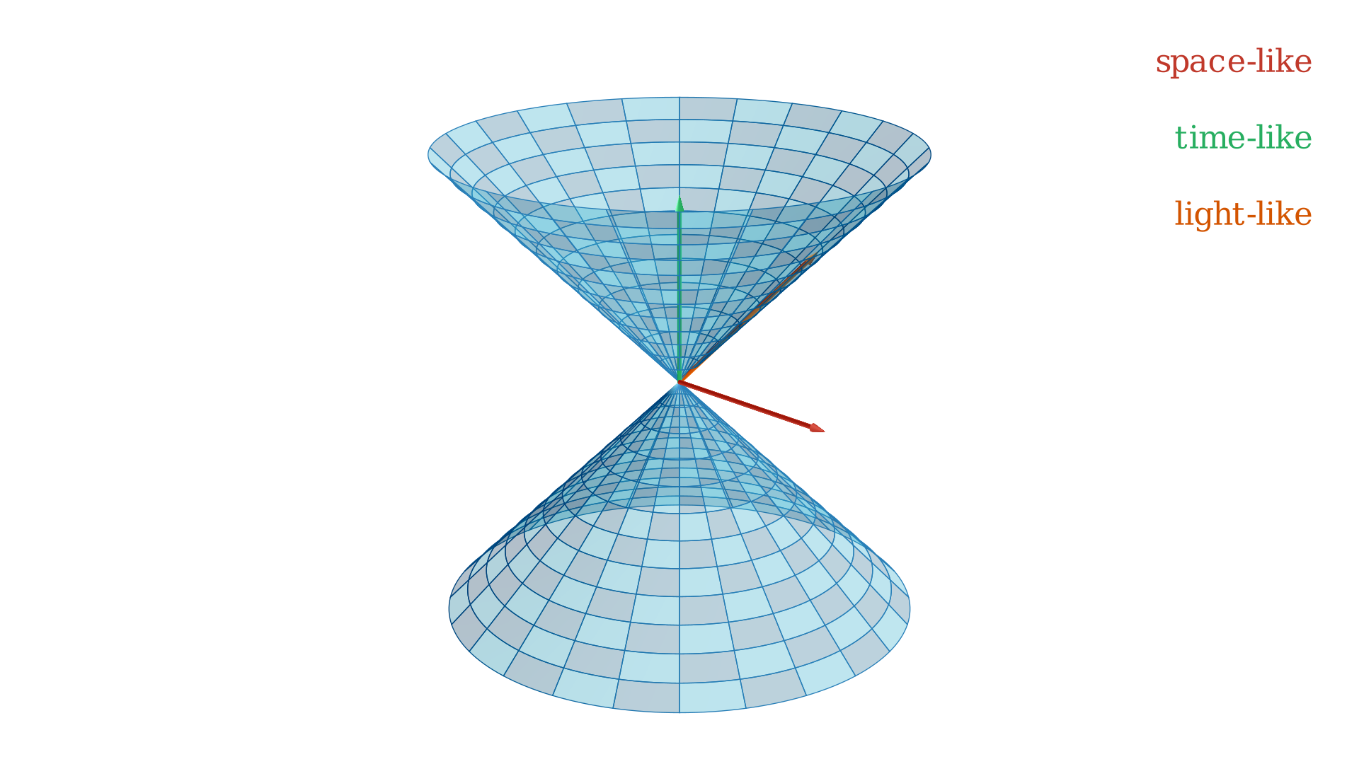
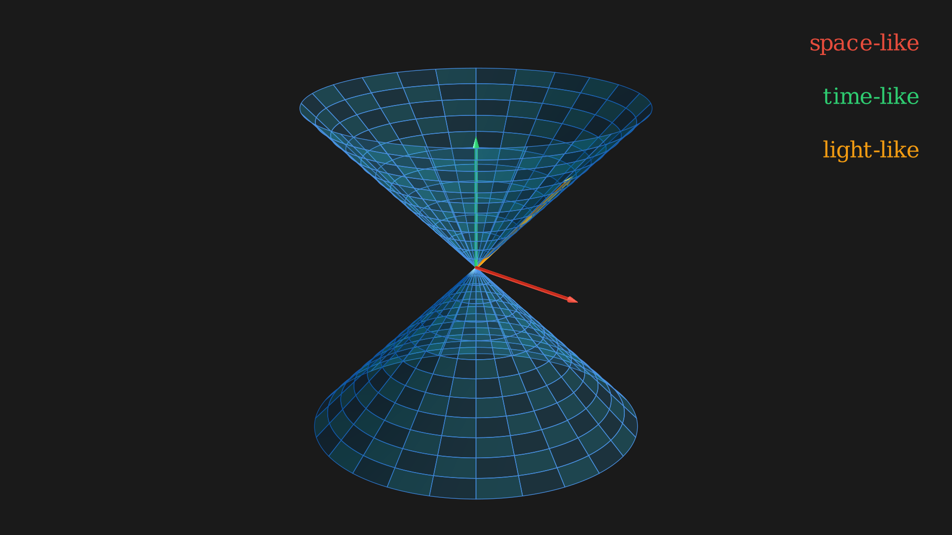
Generally, given a state $(x, t), (p,s)$ with timelike momentum ( $|p|^2 - s^2 < 0$) we have the mass of the state to be $m = \sqrt{-(|p|^2 - s^2)}$. It is very interesting that the only thing we need to do for incorporating relativity is enlarge the phase space by two dimensions and use the Lorentzian metric which is still quadratic. But the Lorentzian metric is not positive definite, so instead of having unit cospheres which are compact (Figure ) they will look like hyperboloids and be non-compact.

What this means is if $X=\mathbb{R}^3$, $g_X = dx^2 + dy^2 + dz^2$ then the system $(\hat{X} = \mathbb{R}^3 \times \mathbb{R}, g_{\text{Lorentzian}}=g_X - dt^2)$ has an enlarged group of symmetries including the famous Poincaré group (translation in space and time, rotations in space, and boosts, or changes in velocity). This would look like $SO(3, 1)\ltimes \mathbb{R}^4$ where $\ltimes$ is the semidirect product; these all preserve the Lorentzian metric.

References and Footnotes

1. Even if you think you are a bit fuzzy on some of them, you should be able to go through them as they appear in the article. ↩

2. Why is there a projection? By how we built the state space, a point of $T^*X$ is a pair $(q,p)$ with $q\in X$ and $p$ a covector at $q$. So there is a natural “forgetful” map that just returns the base point: $\pi(q,p)=q$. In the case $T^*S^1\cong S^1\times\mathbb{R}$, this is simply the first coordinate. ↩

3. Or how the state of the system evolves in time. ↩

4. The Poisson bracket is a way to define a Lie bracket on the space of functions on the state space. ↩

5. Interestingly, there are also higher degree variants or multi-symplectic structures $\omega \in \Omega^k(M)$ for $k \geq 2$. ↩