An Intuitive Look at the Dynamics of SGD

This blog post is an intuitive look through the chronicles of Stochastic Gradient Descent (SGD), one of the most popular algorithms. I try to explain the reasoning behind some of the interesting aspects of SGD, like the stochastic gradient noise, the SGN covariance matrix, and SGD’s preference for flat minima. Recently, I’ve found it fascinating to explore and draw parallels with learning dynamics of algorithms based on gradient descent. Some ideas have particularly taken a bit of time for me to truly understand and with this, I hope to make it easier for others.

But first…

Let’s take a quick look at Stochastic Gradient Descent (SGD).

We consider the data samples $x = \{x_j\}_{j=1}^m$ and similarly $y = \{y_j\}_{j=1}^m$, the model parameters $\theta$, and some loss function $L(\theta, x, y)$. And following popular literature, for brevity, we denote the training loss as $L(\theta)$. We have SGD as follows:

\[\tag{1}\theta_{t+1} = \underbrace{\theta_t}_{\substack{\text{previous}\\\text{params}}} - \overbrace{\eta}^{\text{step-size}} \frac{\partial\overbrace{\hat{L}(\theta_t, x, y)}^{\substack{\text{stochatic estimate}\\\text{of loss}}}}{\partial\underbrace{\theta_t}_{\substack{\text{previous}\\\text{params}}}}\]

where $\eta$ is the step size, and $\hat{L}(\theta_t, x, y)$ is the stochastic estimate of the loss function.

We can then use the noise induced by the noisy estimates of the true gradient, we can rewrite this in terms of the stochastic gradient noise covariance as follows, taken directly from ¹:

\[\tag{2}\theta_{t+1} = \theta_t - \eta \nabla L(\theta_t) + \eta\underbrace{C(\theta_t)^{\frac{1}{2}}}_{\substack{\text{SGN}\\ \text{covariance}}}\overbrace{\zeta_t}^{\substack{\text{standard }\mathcal{N}\\ \text{random}\\ \text{variable}}}\]

where $\hat{L}_S(\theta)=\frac{1}{S}\sum_{n \in \mathcal{S}}\ell^{(n)}(\theta)$ is the stochastic estimate of the loss function, $\mathcal{S}$ is a minibatch of size $S$, $\zeta_t \sim \mathcal{N}(0, I)$ is a standard normal random variable, and $C(\theta_t)$ is the stochastic gradient noise (SGN) covariance matrix.

Notice that, the stochastic gradient noise is simply introduced by the minibatch aspect of SGD and is the difference between gradient descent and SGD, so we have:

\[\tag{3}C(\theta_t)^{\frac{1}{2}}\zeta_t = \underbrace{\frac{\partial L(\theta_t)}{\partial \theta_t}}_{\substack{\text{gradient}\\\text{descent}}} - \underbrace{\frac{\partial \hat{L}(\theta_t)}{\partial \theta_t}}_{\text{SGD}}\]

And this is a quick recap of the standard well-known aspects of SGD. And now let’s move on to some of the interesting aspects of the learning dynamics. Let’s start by talking about the SGN component.

Modelling the Stochastic Gradient Noise (SGN)

The stochastic gradient noise (SGN) is significant in SGD, and it is important to model it. Firstly, the convergence properties of SGD are fundamentally influenced by the characteristics of SGN. An accurate model of this noise allows for a more nuanced understanding of the convergence dynamics, especially in complex optimization landscapes typical of high-dimensional deep-learning tasks. A popular example is that SGN provides the necessary stochasticity to escape sharp minima, this escape is facilitated by the noise-enabling gradient updates that move the parameters out of these steep curvature regions, thus promoting convergence to broader, flatter minima which are less sensitive to data variations and hence generalize better. Theoretical models that accurately capture the behavior of SGN can provide insights into the conditions under which SGD converges to a minimum and the rate at which this convergence occurs. Furthermore, the SGN component intuitively achieves a regularizing effect, we can view the stochastic nature of gradient updates as performing an implicit averaging over different directions in the gradient space. Accurate modeling of SGN can inform more effective strategies for hyperparameter tuning, optimizing the performance of the learning algorithm.

Theorem (Gnedenko-Kolmogorov Generalized Central Limit):

For a sequence of independent random variables $X_1, X_2, \ldots, X_n$ with a common distribution that has an infinite variance, the normalized sum

\[\tag{4}Z_n = \frac{1}{n^{\frac{1}{\alpha}}} \sum_{i=1}^{n} X_i\]

converges in distribution to a stable distribution as $n \rightarrow \infty$, where $0 < \alpha \leq 2$ is the index of the stable distribution.

With the generalized central limit theorem ², we know that a non-degenerate random variable $Z$ is $\alpha$-stable for some $\alpha \in (0,2]$ if and only if there is an independent, identically distributed sequence of random variables $X_1, X_2, \ldots X_n$ and some constants $a_n > 0$ and $b_n \in \mathbb{R}$ such that $a_n(X_1+X_2+\ldots+X_n)-b_n \rightarrow Z$. So, the mean of many infinite-variance random variables converges to a stable distribution, while the mean of many finite-variance random variables converges to a Gaussian distribution. Thus, it is reasonable to model the stochastic gradient noise as approximately Gaussian, $\zeta_t \sim \mathcal{N}(0, I)$.

There have been some works like ³$^,$⁴ have shown that the stochastic gradient noise is heavy-tailed, and thus the Gaussian assumption is not valid, instead the SGN is close to a stable distribution. However, we can see empirical evidence that the SGN is approximately Gaussian in the following figures. You can observe that for smaller batch sizes it is quite hard to conclude what the SGN models to. These plots are produced by training ResNet18 on MNIST.

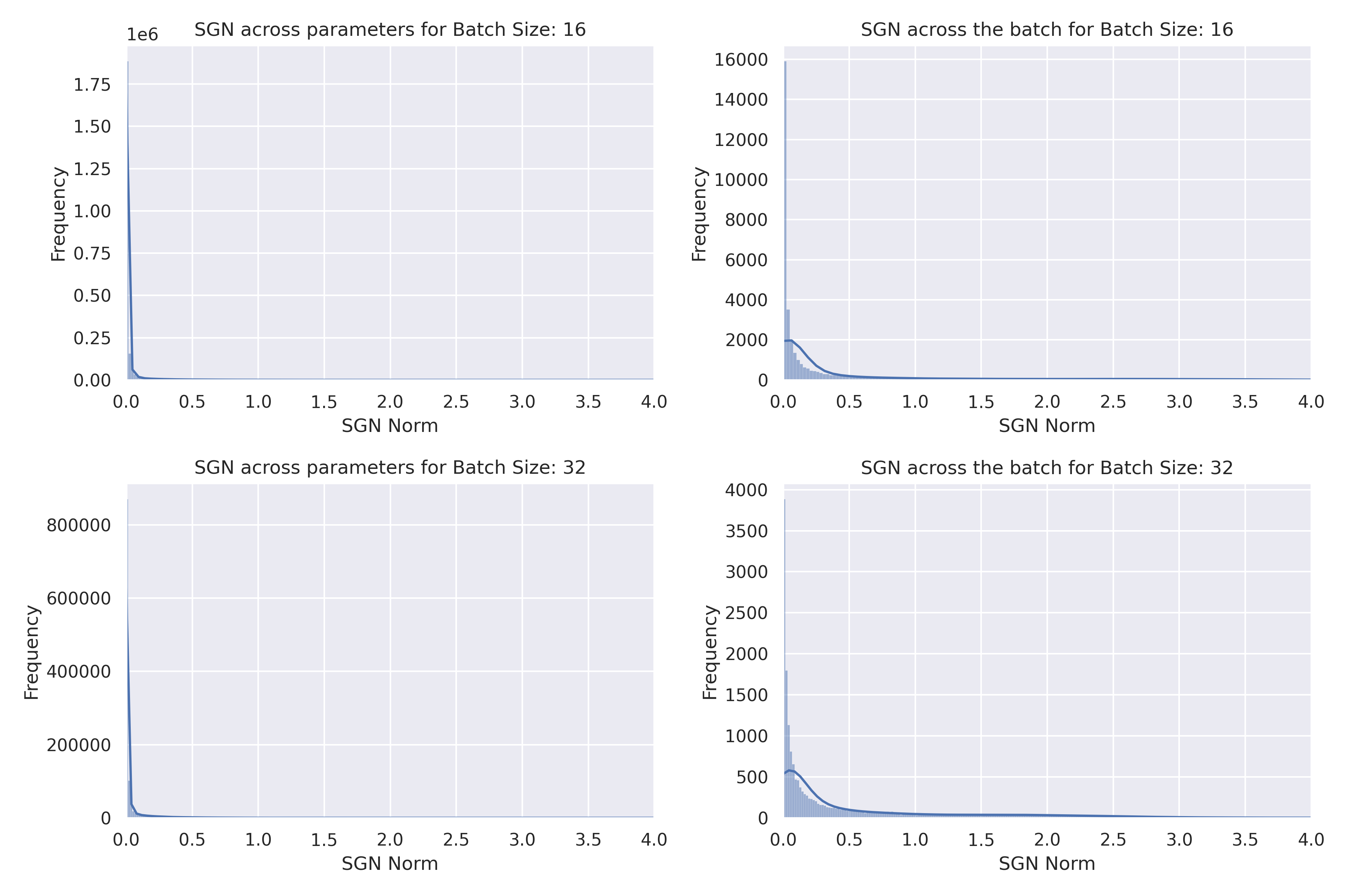
Figure: Histogram of the SGN computed across parameters and SGN computed across batches. These are generated by training ResNet18 on MNIST for batch sizes: 16, and 32 (note the axes).

However, for larger batch sizes, we can see that the SGN computed across batches is indeed approximately Gaussian, empirically, and not heavy-tailed Stable distribution when computing the SGN norm across batches. It is also apparent that the stochastic gradient computed across parameters is approximately a heavy-tailed Stable distribution. Notice that it is possible for the stochastic gradient across parameters to be a heavy-tailed Stable distribution, while the SGN across batches is approximately Gaussian since we couldn’t possibly assume the SGN to be isotropic.

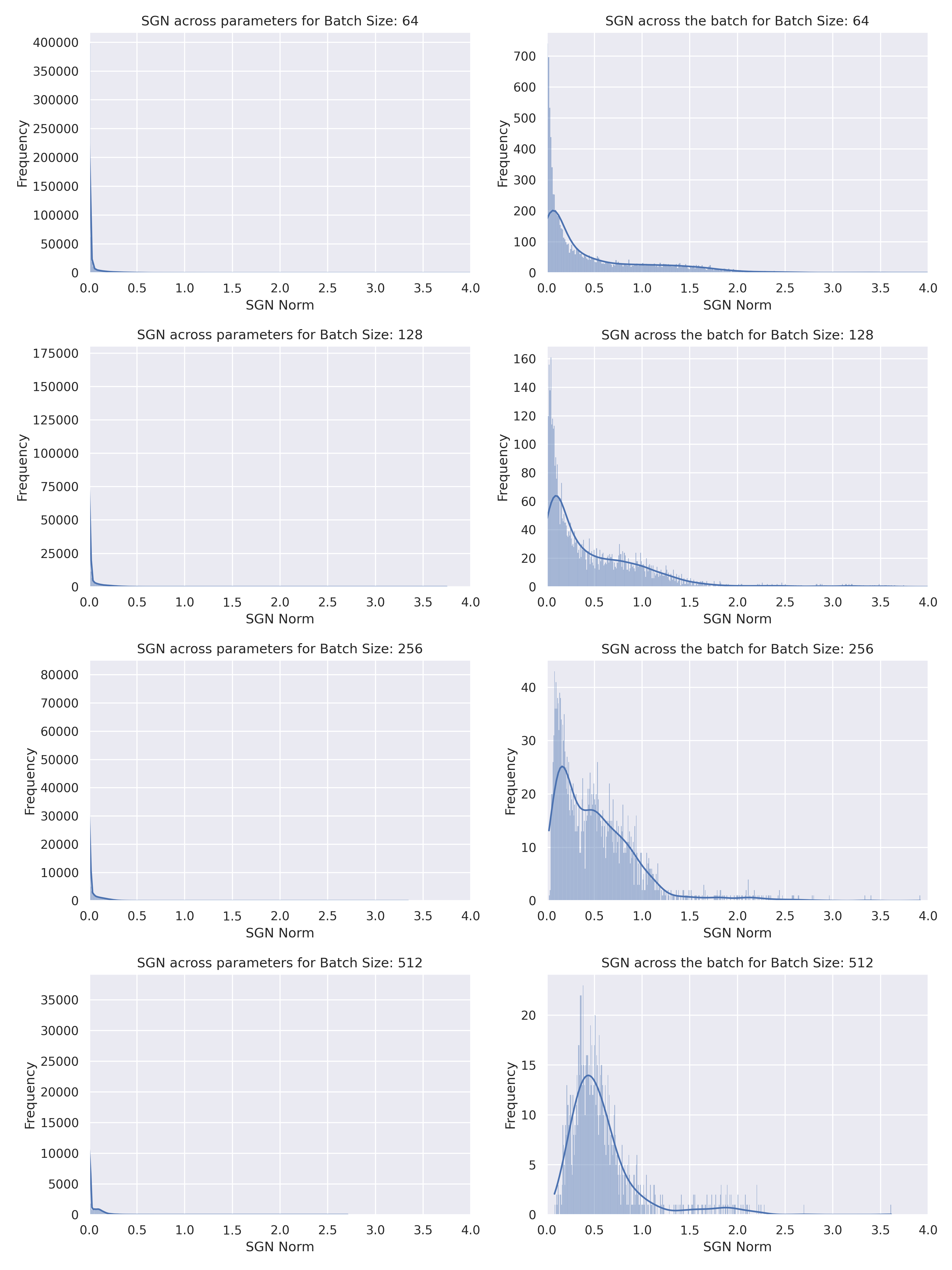
Thus it makes sense to model the SGN, which is an important aspect of what SGD learns, as approximately Gaussian for larger batch sizes.

SGD can reach multiple minima

Before talking about kinds of minima at all, we can first identify that for a lot of non-convex problems there is no guarantee what kind of minima SGD would reach too. We could for instance (in the way we describe), change the batch size and step size to reach different minima. A question does arise, which minima would we ideally choose?

We are interested in a large region of connected acceptable minima, where each weight $w$ within this region leads to almost identical net functions $\text{net}(w)$. Such a region is called a flat minimum.

– Hochreiter and Schmidhuber ⁵$^,$⁶

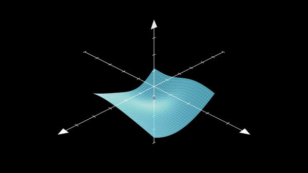
Ideally, we want to be in a flat minima:

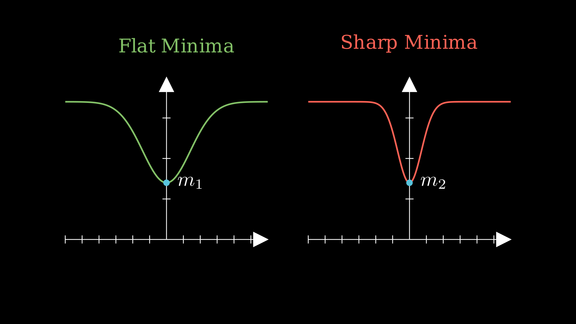
Figure: An intuitive informal comparison of flat minima vs sharp minima

If you just take a look at the above images, if we do end up in a sharp minima, even a little distribution shift in the training data affects the training loss by a big margin, and we want to end up in a flat minima even if the training loss is higher than a sharp minima, due to the robustness. However, reaching a flat minima does not guarantee generalization and is not a necessary condition for better generalization, ⁷ showed that we can reparemeterize a neural network and make a sharp minima look like a flat minima.

Interestingly, SGD learns to reach or prefers reaching a flat minima, which might seem a bit counterintuitive at first, so we do want to take a look at why this might happen.

This is not the case with standard gradient descent (gradient descent does not necessarily prefer a flat/wide minima), but SGD does. Thus, a good place to start is the SGN component, we had that the SGN is:

\[\tag{5}\begin{aligned}U_k(\theta) &\overset{\Delta}{=} \nabla\hat{L}_k(\theta) - \nabla L(\theta) \\&= \frac{1}{S}\sum_{i \in \mathcal{S}} \left[ \nabla \ell^{(i)}(\theta) - \nabla L(\theta) \right]\end{aligned}\]

What affects the SGN covariance matrix?

Let us now try to see a relation to what affects the SGN covariance matrix.

Theorem (SGN Covariance Matrix):

The SGN Covariance $C(\theta)\propto\frac{\overbrace{\mathbf H_\theta}^{\text{Hessian}}}{\underbrace{S}_{\text{batch-size}}}$ where $\mathbf H_\theta$ represents the Hessian matrix and $S$ represents the batch-size ⁸.

Proof (for a large part follows the proof in ⁸):

Note: We can easily prove this empirically, but that holds very little weight. It is well known that Neural Networks at scale always seem to outperform theory, so empirical proof is necessary but not sufficient to convince us enough.

In the earlier section, we also said $U_t(\theta) \sim \mathcal{N}(0, \sigma^2\mathbf I)$.

Now considering this, we can write the update rule recursively as follows:

\[\tag{6}\begin{aligned} \theta_{t+1} &= \theta_t - \eta \nabla L(\theta_t) + \left(\eta C(\theta_t)\right)^{\frac{1}{2}}\zeta_t\\ &= \theta_t - \eta \nabla L(\theta_t) + U_t(\theta)\\ &= \underbrace{\theta_t}_{\substack{\text{previous}\\\text{weight}}} - \underbrace{\eta}_{\text{step-size}} \nabla L(\theta_t) + \sqrt{\eta} \sqrt{\eta\sigma^2}\underbrace{Z_t}_{\substack{\text{standard } \mathcal{N}\\ \text{random variable}}} \end{aligned}\]

For a small step size, we can now see that we can write this step-wise update rule as a discretization of this continuous-time stochastic differential equation (SDE - It$\hat{\text{o}}$ SDE), and the solutions for this SDE would be Markov processes, as follows:

\[\tag{7}\begin{aligned}\operatorname{d}\theta &= -\nabla L(\theta)\operatorname{d}t + \sqrt{n\sigma^2}\underbrace{\operatorname{d}B_t}_{\substack{\text{standard Brownian}\\\text{motion}}} \\&= - \frac{\partial L(\theta)}{\partial \theta}\operatorname{d}t + [2D(\theta)]^{\frac{1}{2}}\operatorname{d}B_t \end{aligned}\]

We replace $\eta$ by $\operatorname{d}t$ as unit time, say $\operatorname{d}B_t \sim \mathcal{N}(0,\mathbf I \operatorname{d}t)$, and $D(\theta)=\frac{\eta}{2}C(\theta)$.

And you can observe that if you just discretize Equation 7 with the $\eta$, we get the update rule in Equation 6. And drawing inspiration from a lot of statistical physics problems we can try to study Equation 7 and use findings from there to understand SGD better. Intuitively, Equation 7 tells us that the update of the parameters in SGD is a combination of a deterministic move in the direction of the gradient (trying to reduce the loss) and a stochastic move that adds randomness.

Now, we can focus on understanding Equation 7. Let’s define some probability density function $p(\theta, t)$ over time. We can write the Fokker-Planck equation for this probability density function as follows, considering $\theta$ is an $N$-dimensional vectors, $[2D(\theta)]^{\frac{1}{2}}$ is some $N \times M$ matrix, and $B_t$ is the standard $M$-dimensional Brownian motion vector:

\[\tag{8}\begin{aligned}\frac{\partial p(\theta, t)}{\partial t} &= \nabla\cdot\left[p(\theta, t)\nabla L(\theta)\right] + \nabla\cdot\nabla D(\theta)p(\theta, t)\\ &= \underbrace{\overbrace{\sum_i \frac{\partial}{\partial \theta_i}}^{\substack{\text{consider changes}\\\text{in } p \text{ across}\\\text{all dimensions}}} \Biggl[ p(\theta, t) \overbrace{\frac{\partial L(\theta)}{\partial \theta_i}}^{\substack{\text{drift}\\\text{vector}}} \Biggr]}_{\text{drift term}} + \underbrace{\overbrace{\sum_i \sum_j \frac{\partial^2}{\partial \theta_i \partial \theta_j}}^{\substack{\text{diffusion across}\\\text{all pairs}\\\text{of dimensions}}} [\overbrace{D_{ij}(\theta)}^{\substack{\text{diffusion}\\\text{tensor}}} p(\theta, t)]}_{\text{diffusion term}} \end{aligned}\]

In this example, of Fokker-Planck, we can consider $\nabla L(\theta)$ as the drift vectors and $\sigma(\mathbf X_t, t) = \left[2D(\theta)\right]^{\frac{1}{2}}$. From Equation 8, we can think of it as: a higher diffusion constant leads to a faster spreading of the probability density, indicating a more rapid diffusion of the state through the state space. Remember, we also had $D(\theta)=\frac{\eta}{2}C(\theta)$.

⁹$^,$⁸ showed that Equation 9 made for a good approximation of the SGN covariance matrix $C(\theta)$,

\[\tag{9}C(\theta)\approx\frac{1}{Sm}\sum_{j=1}^{m}\nabla L(\theta, x_j)L(\theta, x_j)^\top\]

This makes for an interesting proof, but instead, here we try to see why this makes for a good approximation. Instead of considering the exact noise distribution, which is computationally expensive, we estimate it by averaging over the outer products of the mini-batch gradients, this approximation captures the variance of the stochastic gradient near the critical points. It also simplifies computation by using only the gradients from the current mini-batch rather than requiring additional computations over multiple mini-batches or the whole dataset.

The Fisher Information $I$ is defined as the expected outer product of the gradient of the log-likelihood with respect to $\theta$,

\[I(\theta) = \mathbb{E} [\underbrace{\nabla \log L(\theta, x) }_{\text{score function}}\nabla \log L(\theta, x)^\top]\]

If we consider the gradients computed on the mini-batches as samples from the distribution of gradients, then the outer product of these gradients is a sample estimate of the Fisher Information, $C(\theta) = \frac{I(\theta)}{S}$.

Furthermore, near a minimum, the loss function can be approximated by a second-order Taylor expansion, $L(\theta + \delta) \approx L(\theta) + \delta^\top \nabla L(\theta) + \frac{1}{2} \delta^\top \mathbf H_\theta \delta$. At the minima, $\nabla L(\theta) = 0$, and the quadratic term with the Hessian dominates. Near a minimum, the loss function is approximately quadratic, and the Hessian captures the curvature of this quadratic bowl. If the loss function $L(\theta)$ is taken to be the negative log-likelihood, then the Hessian of the loss is related to the negative of the expected outer product of the gradient of the log-likelihood, which is the $I$.

So, near a minimum we have, $\mathbb{E}[H_\theta] = -\mathbb{E}\left[\nabla_{\theta}^2 \log p(x\mid\theta)\right] = I(\theta)$, and thus $\mathbf H_\theta\approx I(\theta)$.

\[\tag{10}C(\theta)\approx\frac{\overbrace{\mathbf H_\theta}^{\text{Hessian}}}{\underbrace{S}_{\text{batch-size}}}\]

One of the main implications of the Theorem (SGN Covariance Matrix), in terms of sharp and flat minima, is that the gradient noise also depends on the curvature of the loss function. In regions where the loss function is sharply curved (high values in the Hessian), we expect more noise in the gradient estimates. This is because small changes in parameters can lead to larger changes in the gradient, making the gradient estimate more sensitive to the specific samples chosen in the mini-batch.

SGD chooses a flat minima

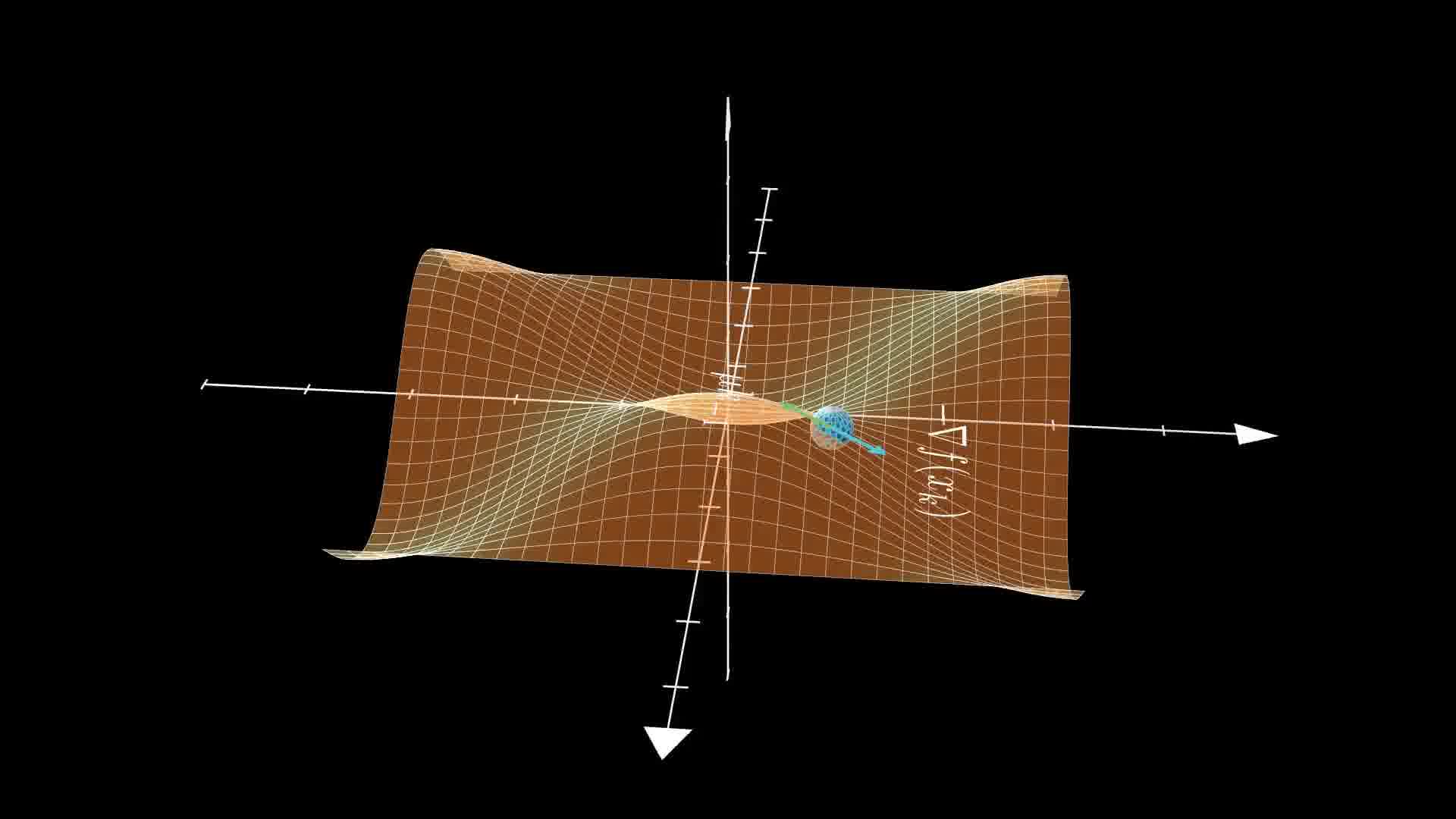
Understanding what kind of minima SGD prefers is a classic case of the popular Kramer’s Escape problem. The mean escape time $\tau$ is the time it takes (for our SGD) to move from a steep valley to a flat valley which contains a flat minima. The figure below shows exactly the problem at hand:

Now, I mainly follow the works by ¹⁰$^,$⁸ and write:

\[\tag{11}\underbrace{\tau}_{\substack{\text{mean escape}\\\text{time}}} = \frac{\overbrace{\int_{\underbrace{V_s}_{\substack{\text{volume}\\\text{surrounded}\\ \text{by }S_s}}}P(\theta)dV}^{\substack{\text{current probability}\\\text{inside the steep valley}}}}{\underbrace{\int_{\underbrace{S_s}_{\substack{\text{surface}\\\text{surrounding}\\\text{steep valley}}}}J\cdot dS}_{\substack{\text{rate at which}\\\text{it escapes}}}}\]

where $J$ is the probability current, which makes sense since we are roughly saying that $\tau$ is the ratio of the total probability inside the valley to the rate at which it’s escaping (probability flux).

The relation holds true for any valley $s$, I just write “steep valley” in the above equation to make it clearer in the context of Kramer’s Escape problem.

These hold under a few assumptions: that the Second Order Taylor approximation which we also used earlier holds (one might think in a steep valley if the Hessian $\mathbf H_\theta$ changes rapidly, Taylor approximation would not be so good, however, this is related to the other assumptions), quasi-equilibria which means that near a minima the systems would approximately be in equilibrium (a common measure of this could be gradients being very small, but this differs in systems, for example for Langevin dynamics would imply that the dynamics are dominated by small fluctuations around the equilibrium state), and low-temperature which here means that the $D = \frac{\eta}{2S} \mathbf H_\theta$, and thus the accompanying gradient noise is reasonably small.

Theorem (SGN Escapes a Steep Minima):

The loss function $L(\theta)$ is of class $C^2$ and $n$-dimensional. Only one most possible path exists between Valley a and outside of Valley a. If Assumptions hold, and the dynamics are governed by SGD, the mean escape time from Valley a to the outside of Valley a is

\[\tau = 2 \pi \frac{1}{\mid\mathbf H_{be}\mid}\exp(\left[\frac{2S\Delta L}{\eta}\left(\frac{s}{\mathbf H_{ae}}\right)+\frac{1-s}{\mid\mathbf H_{be}\mid}\right])\]

where $S\in(0,1)$ is a path-dependent parameter, and $\mathbf H_{ae}$ and $\mathbf H_{be}$ are, respectively, the eigenvalues of the Hessians at the minimum $a$ and the saddle point $b$ corresponding to the escape direction $e$.

Proof:

Check out ¹¹ for this theorem and proof and ¹⁰ to better understand the proof.

The theorem formally defines the most possible path (MPP) as: the gradient perpendicular to the path direction must be zero, and the second-order directional derivatives perpendicular to the path direction must be non-negative. This particularly means that the MPP is actually the path that has a high loss saddle point and thus is the path we want to use to get out of the steep minima (you can see how this might be helpful in the steep minima visualization as well).

We can say that $\tau$ is not just a measure of duration but also an indicator of SGD’s preference for certain types of minima. Furthermore, the eigenvalues of the Hessian at a given point (like a minimum or saddle point) indicate the nature of the curvature in different directions. Large eigenvalues imply a steep curvature, while small eigenvalues indicate a flatter curvature.

Now from the Theorem, we can observe that SGD is less likely to remain in steep minima due to the shorter escape times associated with them. Conversely, areas with longer escape times—typically flatter minima—pose more of a ‘trap’ for SGD. This ‘trapping’ effect suggests that, over time, SGD is more likely to be found in flatter regions of the loss landscape. So we do have that the SGD exponentially favors a flat/wide minima over a sharp minima.

Concluding Thoughts

I did try quite a few experiments with multiple variants of ResNets on simple and complex datasets, however, it does become a bit harder to quantitatively understand the mean escape time. This is most likely because increasing to quite a lot of dimensions probably makes many escape paths. Now even if we do have multiple valleys we can move to, all we need is a saddle point that connects two valleys. Thus, you would have a reduced mean escape time.

Lately understanding some of these aspects of learning dynamics for gradient descent-based algorithms has been quite interesting, though some ideas about the effect of SGN, choosing minima, and others have taken me a bit of time or made it harder to understand the intuition behind them. I hope this blog post helps you understand these aspects of learning too!

References

Stephan, M., Hoffman, M. D., & Blei, D. M. (2017). Stochastic gradient descent as approximate bayesian inference. Journal of Machine Learning Research, 18(134), 1-35. ↩
Lindley, D. V. (12 2018). Limit Distributions for Sums of Independent Random Variables. Royal Statistical Society. Journal. Series A: General, 118(2), 248–249. doi:10.2307/2343136 ↩
Simsekli, U., Sagun, L., & Gurbuzbalaban, M. (2019, May). A tail-index analysis of stochastic gradient noise in deep neural networks. In International Conference on Machine Learning (pp. 5827-5837). PMLR. ↩
Nguyen, T. H., Simsekli, U., Gurbuzbalaban, M., & Richard, G. (2019). First exit time analysis of stochastic gradient descent under heavy-tailed gradient noise. Advances in neural information processing systems, 32. ↩
Hochreiter, S., & Schmidhuber, J. (1997). Flat minima. Neural computation, 9(1), 1-42. ↩
Hochreiter, S., & Schmidhuber, J. (1994). Simplifying neural nets by discovering flat minima. Advances in neural information processing systems, 7. ↩
Dinh, L., Pascanu, R., Bengio, S., & Bengio, Y. (2017, July). Sharp minima can generalize for deep nets. In International Conference on Machine Learning (pp. 1019-1028). PMLR. ↩
Xie, Z., Sato, I., & Sugiyama, M. (2020). A diffusion theory for deep learning dynamics: Stochastic gradient descent exponentially favors flat minima. arXiv preprint arXiv:2002.03495. ↩ ↩² ↩³ ↩⁴
Smith, S. L., & Le, Q. V. (2017). A bayesian perspective on generalization and stochastic gradient descent. arXiv preprint arXiv:1710.06451. ↩
Paquette, C., Lee, K., Pedregosa, F., & Paquette, E. (2021, July). SGD in the large: Average-case analysis, asymptotics, and stepsize criticality. In Conference on Learning Theory (pp. 3548-3626). PMLR. ↩ ↩²
Hu, W., Li, C. J., Li, L., & Liu, J. G. (2017). On the diffusion approximation of nonconvex stochastic gradient descent. arXiv preprint arXiv:1705.07562. ↩