The Art of Hyperparameter Tuning in Deep Neural Nets by Example

Hello developers 👋, If you have worked on building Deep Neural Networks earlier you might know that building neural nets can involve setting a lot of different hyperparameters. In this article, I will share with you some tips and guidelines you can use to better organize your hyperparameter tuning process which should make it a lot more efficient for you to stumble upon a good setting for the hyperparameters.
What is a hyperparameter anyway?🤷♀️
Very simply a hyperparameter is external to the model that is it cannot be learned within the estimator, and whose value you cannot calculate from the data.
Many models have important parameters which cannot be directly estimated from the data. This type of model parameter is referred to as a tuning parameter because there is no analytical formula available to calculate an appropriate value.
— Page 64, 65, Applied Predictive Modeling, 2013
The hyperparameters are often used in the processes to help estimate the model parameters and are often to be specified by you. In most cases to tune these hyperparameters, you would be using some heuristic approach based on your experience, maybe starter values for the hyperparameters or find the best values by trial and error for a given problem.
As I was saying at the start of this article, one of the painful things about training Deep Neural Networks is the large number of hyperparameters you have to deal with. These could be your learning rate \(\alpha\), the discounting factor ρ, and epsilon ϵ if you are using the RMSprop optimizer (Hinton et al.) or the exponential decay rates \(\beta\)₁ and \(\beta\)₂ if you are using the Adam optimizer (Kingma et al.). You also need to choose the number of layers in the network or the number of hidden units for the layers, you might be using learning rate schedulers and would want to configure that and a lot more😩! We definitely need ways to better organize our hyperparameter tuning process.
Which hyperparameters are more important?📑
Usually, we can categorize hyperparameters into two groups: the hyperparameters used for training and those used for model design🖌️. A proper choice of hyperparameters related to model training would allow neural networks to learn faster and achieve enhanced performance making the tuning process, definitely something you would want to care about. The hyperparameters for model design are more related to the structure of neural networks a trivial example being the number of hidden layers and the width of these layers. The model training hyperparameters in most cases could well serve as a way to measure a model’s learning capacity🧠.
During the training process, I usually give the most attention to the learning rate \(\alpha\), and the batch size because these determine the speed of convergence so you should consider tuning them first or give them more attention. However, I do strongly believe that for most models the learning rate \(\alpha\) would be the most important hyperparameter to tune consequently deserving more attention. We will later in this article discuss ways to select the learning rate. Also do note that I mention “usually” over here, this could most certainly change according to the kind of applications you are building.
Next up, I usually consider tuning the momentum term \(\beta\) in RMSprop and others since this helps us reduces the oscillation by strengthening the weight updates in the same direction, also allowing us to decrease the change in different directions. I often suggest using \(\beta = 0.9\) which works as a very good default and is most often used too.
After doing so I would try and tune the number of hidden units for each layer followed by the number of hidden layers which essentially help change the model structure followed by the learning rate decay which we will soon see. Note: The order suggested in this paragraph has seemed to work well for me and was originally suggested by Andrew Ng.
Furthermore, a really helpful summary about the order of importance of hyperparameters from lecture notes of Ng was compiled by Tong Yu and Hong Zhu in their paper suggesting this order:
-
learning rate
-
Momentum \(\beta\), for RMSprop, etc.
-
Mini-batch size
-
Number of hidden layers
-
learning rate decay
-
Regularization \(\lambda\)
Common approaches for the tuning process🕹️
The things we talk about under this section would essentially be some things I find important and apply while the tuning of any hyperparameter. So, we will not be talking about things related to tuning for a specific hyperparameter but concepts that apply to all of them.
Random Search
Random Search and Grid Search (a pre-cursor of Random Search) are by far the most widely used methods because of their simplicity. Earlier it was very common to sample the points in a grid and then systematically perform an exhaustive search on the hyperparameter set specified by users. And this works well and is applicable for several hyperparameters with limited search space. In the diagram here as we mention Grid Search asks us to systematically sample the points and try out those values after which we could choose the one which best suits us.
](/assets/the-art-of-hyperparameter-tuning-in-deep-neural-nets-by-example/search.png)
To perform hyperparameter tuning for deep neural nets it is often recommended to rather choose points at random. So in the image above, we choose the same number of points but do not follow a systemic approach to choosing those points like on the left side. And the reason you often do that is that it is difficult to know in advance which hyperparameters are going to be the most important for your problem. Let us say the hyperparameter 1 here matters a lot for your problem and hyperparameter 2 contributes very less you essentially get to try out just 5 values of hyperparameter 1 and you might find almost the same results after trying the values of hyperparameter 2 since it does not contribute a lot. On other hand, if you had used random sampling you would more richly explore the set of possible values.
So, we could use random search in the early stage of the tuning process to rapidly narrow down the search space, before we start using a guided algorithm to obtain finer results that go from a coarse to fine sampling scheme. Here is a simple example with TensorFlow where I try to use Random Search on the Fashion MNIST Dataset for the learning rate and the number of units:
import kerastuner as kt
import tensorflow as tf

def model_builder(hp):
  model = tf.keras.Sequential()
  model.add(tf.keras.layers.Flatten(input_shape=(28, 28)))

  # Tune the number of units in the first Dense layer
  # Choose an optimal value between 32-512
  hp_units = hp.Int('units', min_value = 32, max_value = 512, step = 32)
  model.add(tf.keras.layers.Dense(units = hp_units, activation = 'relu'))
  model.add(tf.keras.layers.Dense(10))

  # Tune the learning rate for the optimizer
  # Choose an optimal value from 0.01, 0.001, or 0.0001
  hp_learning_rate = hp.Choice('learning_rate', values = [1e-2, 1e-3, 1e-4])

  model.compile(optimizer = tf.keras.optimizers.Adam(learning_rate = hp_learning_rate),
                loss = tf.keras.losses.SparseCategoricalCrossentropy(from_logits = True),
                metrics = ['accuracy'])

  return model

tuner = kt.RandomSearch(model_builder,
                        objective = 'val_accuracy',
                        max_trials = 10,
                        directory = 'random_search_starter',
                        project_name = 'intro_to_kt')

tuner.search(img_train, label_train, epochs = 10, validation_data = (img_test, label_test))

# Which was the best model?
best_model = tuner.get_best_models(1)[0]

# What were the best hyperparameters?
best_hyperparameters = tuner.get_best_hyperparameters(1)[0]
Hyperband
Hyperband (Li et al.) is another algorithm I tend to use quite often, it is essentially a slight improvement of Random Search incorporating adaptive resource allocation and early-stopping to quickly converge on a high-performing model. Here we train a large number of models for a few epochs and carry forward only the top-performing half of models to the next round.
Early stopping is particularly useful for deep learning scenarios where a deep neural network is trained over a number of epochs. The training script can report the target metric after each epoch, and if the run is significantly underperforming previous runs after the same number of intervals, it can be abandoned.
Here is a simple example with TensorFlow where I try to use Hyperband on the Fashion MNIST Dataset for the learning rate and the number of units:
def model_builder(hp):
  model = keras.Sequential()
  model.add(keras.layers.Flatten(input_shape=(28, 28)))

  # Tune the number of units in the first Dense layer
  # Choose an optimal value between 32-512
  hp_units = hp.Int('units', min_value = 32, max_value = 512, step = 32)
  model.add(keras.layers.Dense(units = hp_units, activation = 'relu'))
  model.add(keras.layers.Dense(10))

  # Tune the learning rate for the optimizer
  # Choose an optimal value from 0.01, 0.001, or 0.0001
  hp_learning_rate = hp.Choice('learning_rate', values = [1e-2, 1e-3, 1e-4])

  model.compile(optimizer = keras.optimizers.Adam(learning_rate = hp_learning_rate),
                loss = keras.losses.SparseCategoricalCrossentropy(from_logits = True),
                metrics = ['accuracy'])

  return model

tuner = kt.Hyperband(model_builder,
                     objective = 'val_accuracy',
                     max_epochs = 10,
                     factor = 3,
                     directory = 'hyperband_starter',
                     project_name = 'intro_to_kt')

tuner.search(img_train, label_train, epochs = 10, validation_data = (img_test, label_test))
Choosing a Learning Rate \(\alpha\)🧐
I am particularly interested in talking more about choosing an appropriate learning rate \(\alpha\) since for most learning applications it is the most important hyperparameter to tune consequently also deserving more attention. Having a constant learning rate is the most straightforward approach and is often set as the default schedule:
optimizer = tf.keras.optimizers.Adam(learning_rate = 0.01)
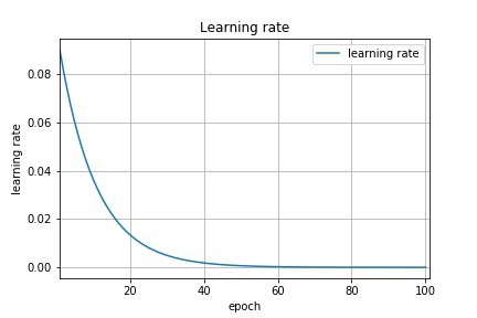
However, it turns out that with a constant LR, the network can often be trained to a sufficient, but unsatisfactory accuracy because the initial value could always prove to be larger, especially in the final few steps of gradient descent. The optimal learning rate would depend on the topology of your loss landscape, which is in turn dependent on both the model architecture and the dataset. So we can say that an optimal learning rate would give us a steep drop in the loss function. Decreasing the learning rate would decrease the loss function but it would do so at a very shallow rate. On other hand increasing the learning rate after the optimal one will cause the loss to bounce about the minima. Here is a figure to sum this up:
](/assets/the-art-of-hyperparameter-tuning-in-deep-neural-nets-by-example/lr.png)
You now understand why it is important to choose a learning rate effectively and with that let’s talk a bit about updating your learning rates while training or setting a schedule. A prevalent technique, known as *learning rate annealing, *is often used, it recommends starting with a relatively high learning rate and then gradually lowering the learning rate📉 during training. As an example, I could start with a learning rate of \(10^{-2}\) when the accuracy is saturated or I reach a plateau we could lower the learning rate to let’s say \(10^{-3}\) and maybe then to \(10^{-5}\) if required.
In training deep networks, it is usually helpful to anneal the learning rate over time. Good intuition to have in mind is that with a high learning rate, the system contains too much kinetic energy and the parameter vector bounces around chaotically, unable to settle down into deeper, but narrower parts of the loss function.
— Stanford CS231n Course Notes by Fei-Fei Li, Ranjay Krishna, and Danfei Xu
Going back to the example above, I suspect that my learning rate should be somewhere between \(10^{-2}\) and \(10^{-5}\) so if I simply update my learning rate uniformly across this range, we use 90% of the resource for the range \(10^{-2}\) to \(10^{-3}\) which does not make sense. You could rather update the LR on the log scale, this allows us to use an equal amount of resources for \(10^{-2}\) to \(10^{-3}\) and between \(10^{-3}\) to \(10^{-4}\). Now it should be super easy for you😎 to understand exponential decay which is a widely used LR schedule (Li et al.). An exponential schedule provides a more drastic decay at the beginning and a gentle decay when approaching convergence.
Here is an example showing how we can perform exponential decay with TensorFlow:
initial_learning_rate = 0.1
lr_schedule = tf.keras.optimizers.schedules.ExponentialDecay(
    initial_learning_rate,
    decay_steps = 100000,
    decay_rate = 0.96,
    staircase = True)

model.compile(optimizer=tf.keras.optimizers.SGD(learning_rate = lr_schedule),
              loss = 'sparse_categorical_crossentropy',
              metrics = ['accuracy'])
Also, note that the initial values are influential and must be carefully determined, in this case, though you might want to use a comparatively large value because it will decay during training.
Choosing a Momentum Term \(\beta\)🧐
To better help us understand why I will later suggest some good default values for the momentum term, I would like to show a bit about why the momentum term is used in RMSprop and some others. The idea behind RMSprop is to accelerate the gradient descent like the precursors Adagrad (Duchi et al.) and Adadelta (Zeiler et al.) but gives superior performance when steps become smaller. RMSprop uses exponentially weighted averages of the squares instead of directly using \(\partial w\) and \(\partial b\):

Now you might have guessed until now the moving average term \(\beta\) should be a value between 0 and 1. In practice, most of the time 0.9 works well (also suggested by Geoffrey Hinton) and I would say is a really good default value. You would often consider trying out a value between 0.9 (averaging across the last 10 values) and 0.999 (averaging across the last 1000 values). Here is a really wonderful diagram to summarize the effect of \(\beta\). Here the:
-
red-colored line represents \(\beta = 0.9\)
-
green-colored line represents \(\beta = 0.98\)
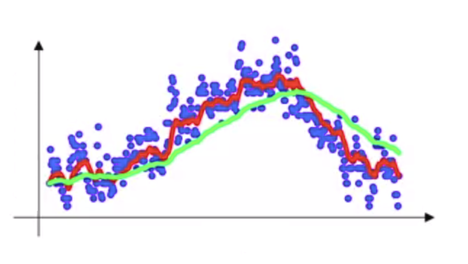
As you can see, with smaller numbers of \(\beta\), the new sequence turns out to be fluctuating a lot, because we’re averaging over a smaller number of examples and therefore are much closer to the noisy data. However with bigger values of beta, like \(\beta\), we get a much smoother curve, but it’s a little bit shifted to the right because we average over a larger number of examples. So in all 0.9 provides a good balance but as I mentioned earlier you would often consider trying out a value between 0.9 and 0.999.
Just as we talked about searching for a good learning rate \(\alpha\) and how it does not make sense to do this in the linear scale rather we do this in the logarithmic scale in this article. Similarly, if you are searching for a good value of \(\beta\) it would again not make sense to perform the search uniformly at random between 0.9 and 0.999. So a simple trick might be to instead search for 1-\(\beta\) in the range 10⁻¹ to \(10^{-3}\) and we will search for it in the log scale. Here’s some sample code to generate these values in the log scale which we can then search across:
r = -2 * np.random.rand() # gives us random values between -2, 0
r = r - 1                 # convert them to -3, -1
beta = 1 - 10**r
Choosing Model Design Hyperparameters🖌️
Number of Hidden Layers d
I will not be talking about some specific rules or suggestions about the number of hidden layers and you will soon understand why I do not do so (by example).
The number of hidden layers d is a pretty critical parameter for determining the overall structure of neural networks, which has a direct influence on the final output. I have seen almost always that deep learning networks with more layers often obtain more complex features and relatively higher accuracy making this a regular approach to achieving better results.
As an example, the ResNet model (He et al.) can be scaled up from ResNet-18 to ResNet-200 by simply using more layers, repeating the baseline structure according to their need for accuracy. Recently, Yanping Huang et al. in their paper achieved 84.3 % ImageNet top-1 accuracy by scaling up a baseline model four times larger!
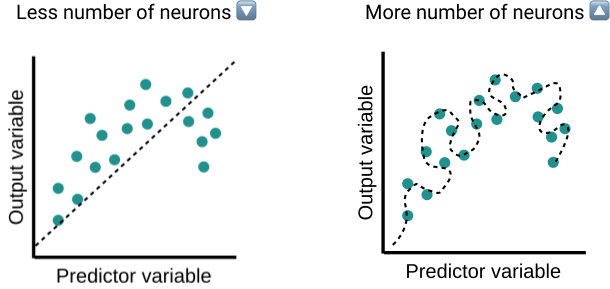
Number of Neurons w
The number of neurons in each layer\(w\)must also be carefully considered after having talked about the number of layers. Too few neurons in the hidden layers may cause underfitting because the model lacks complexity. By contrast, too many neurons may result in overfitting and increase training time.
A couple of suggestions by Jeff Heaton that have worked like a charm could be a good start for tuning the number of neurons. to make it easy to understand here I use \(w_{input}\) as the number of neurons for the input layer and \(w_{output}\) as the number of neurons for the output layer.
-
The number of hidden neurons should be between the size of the input layer and the size of the output layer. \(w_{input}\) <\(w\)< \(w_{output}\)
-
The number of hidden neurons should be 2/3 the size of the input layer, plus the size of the output layer.\(w\)= 2/3 \(w_{input}\) + \(w_{output}\)
-
The number of hidden neurons should be less than twice the size of the input layer. \(w_{input}\) < 2 \(w_{output}\)
And that is it for helping you choose the Model Design Hyperparameters🖌️, I would personally suggest you also take a look at getting some more idea about tuning the regularization \(\lambda\) and has a sizable impact on the model weights if you are interested in that you can take a look at this blog I wrote some time back addressing this in detail: Solving Overfitting in Neural Nets With Regularization
Yeah! By including all of these concepts I hope you can start better tuning your hyperparameters and building better models and start perfecting the “Art of Hyperparameter tuning”🚀. I hope you liked this article.
If you liked this article, share it with everyone😄! Sharing is caring! Thank you!
Many thanks to Alexandru Petrescu for helping me to make this better :)